Taming the AGM

This post is in response to Peter’s post introducing the Approximate Geometric Mean.

The approximate geometric mean $(A G M)$ is a nice approximation of the geometric mean $(G M)$ , but it has some quirks as we will see. After a discussion at the MathsJam gathering, I was intrigued to find out how good an approximation it is.

To get a better understanding, we first have to look again at its definition. For $A = a \cdot 10^{x}$ and $B = b \cdot 10^{y}$ , we set

$A G M (A, B) := A M (a, b) \cdot 10^{A M (x, y)}$

where $A M$ stands for the arithmetic mean. This makes also sense when $a$ and $b$ are not just integers between 1 and 10, but any real numbers. Note that we won’t consider negative $A$ and $B$ (i.e. negative $a$ and $b$ ), as the geometric mean runs into issues if we do so. The values of $x$ and $y$ may be negative, though. The $A G M$ looks like a mix between the $A M$ and the $G M$ , so what can possibly go wrong?

Same mean, different numbers

In contrast to the $A M$ and the $G M$ , the $A G M$ depends on the number base (10 in this case) and the presentation of $A$ and $B$ .

If we write $A = (10 a) \cdot 10^{(x - 1)}$ , we get a different value for $A G M (A, B)$ . This looks rather unfortunate, but it will turn out to be helpful. To ease notation we will assume in the following that $a \geq b$ unless otherwise stated. This can be done without loss of generality as $A G M (A, B) = A G M (B, A)$ .

Peter Rowlett proved in his post that $G M \leq A G M$ . The question is, how far can the $A G M$ exceed the $G M$ ? In other words, what’s the supremum of the ratio $R = A G M / G M$ ?

Using the notation of $A$ and $B$ as above we get
$\begin{aligned} R = \frac{A G M (A, B)}{G M (A, B)} = \frac{A M (a, b)}{G M (a, b)} = \frac{1}{2} \cdot (\sqrt{a / b} + \sqrt{b / a}) . \end{aligned}$

So, the ratio $R$ doesn’t depend on $x$ and $y$ but only on $a$ and $b$ . That’s convenient. Taking $a$ and $b$ in the interval $[1, 10)$ , as is usual, we can look at the plot of $R (a, b)$ .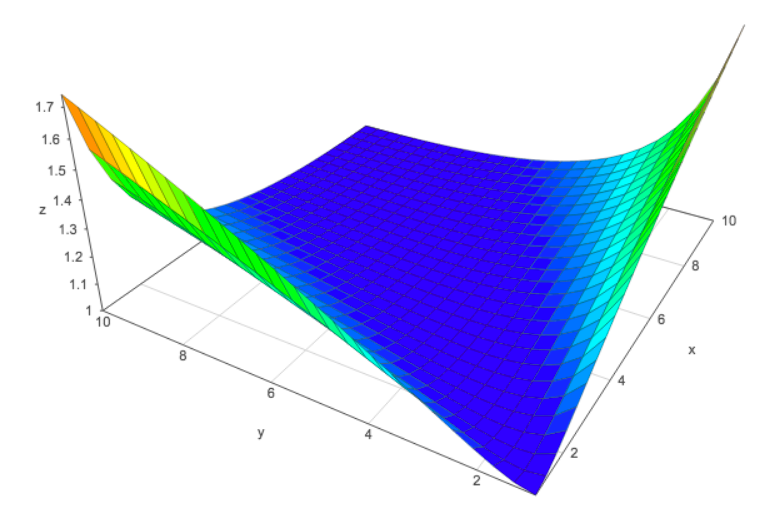

As long as we are in the blue part of the graph, $A G M$ looks to be a sensible approximation of the $G M$ . So let’s look at the bad combinations of $a$ and $b$ .

The worst case happens when $a$ and $b$ are maximally far apart: The supremum of $R (a, b)$ is its limit for $a \to 10$ and $b = 1$ . So in general, $1 \leq R < 5.5 / \sqrt{10} \approx 1.74$ .

This supremum doesn’t look too bad at first, but unfortunately, the result can be unusable in extreme cases. For example, if $a = 999 = 9.99 \cdot 10^{2}$ and $b = 1000 = 1 \cdot 10^{3}$ , we have $G M (A, B) \approx A M (A, B) = 999.5$ and $A G M (A, B) \approx 1738$ – not only is the $A M$ a better approximation of the $G M$ than the $A G M$ in this instance, the $A G M$ is bigger than both the numbers $A$ and $B$ of which it is supposed to give some kind of mean!

Let’s analyse this a bit deeper. The ratio $R$ only depends on the ratio $r = a / b$ . In closed form we can write $R (r) = 1 / 2 \cdot (\sqrt{r} + {\sqrt{r}}^{- 1})$ and we are left to study this function in the range $[1, 10]$ . Its maximum is $R (10)$ , but smaller $r$ give better results. And we will see, that we don’t have to put up with $r = 10$ .

Here, the flexibility of the definition of the $A G M$ comes into play. Due to the choice of a suitable presentation of the numbers we can guarantee that $r$ isn’t too big. If we have $r \leq \sqrt{10}$ which is equivalent to $\sqrt{10} b \geq a \geq b$ we calculate $A G M (A, B)$ as above. If $a > \sqrt{10} b$ , we change the presentation of the number:

$\begin{aligned} B = b \cdot 10^{y} = (10 b) \cdot 10^{y - 1} =: b^{'} \cdot 10^{y - 1} \end{aligned}$
and continue from there.

So, let’s redefine the $A G M$ for $10 > a \geq b \geq 1$ like this:

$A G M (A, B) = {\begin{cases} A M (a, b) \cdot 10^{A M (x, y)}, & \sqrt{10} b \geq a, \\ A M (10 b, a) \cdot 10^{A M (x, y - 1)}, & otherwise . \end{cases}$

Note, that in the second case we have $\sqrt{10} a > 10 b > a$ , so that the roles of the pair $(a, b)$ are taken over by the pair $(10 b, a)$ . Setting $r = 10 b / a$ in the second case, we have in both cases $1 \leq r \leq \sqrt{10}$ , so we only have to study $R (r)$ in the interval $[1, \sqrt{10}]$ , which will turn out to be rather benign.

Note also, that this new $A G M$ can still be calculated without a calculator when using the approximation $\sqrt{10} \approx 3$ , as Colin Beveridge suggested in Peter’s post.

In the example above with $A = 999$ and $B = 1000$ we write $B = 10 \cdot 10^{2}$ and find with this new definition of the $A G M$ :

$\begin{aligned} A G M (999; 1000) = A M (9.99; 10) \cdot 10^{A M (2; 2)} = 999.5, \end{aligned}$

This coincides with the arithmetic mean of the two numbers and is really close to the geometric mean. This is looking promising.

If we define the $A G M$ of two numbers $A$ and $B$ in the way explained above, we get the following two inequalities:

$\begin{aligned} (I) & G M (A, B) \leq A G M (A, B) \leq G M (A, B) \cdot 1.2 \\ (I I) & G M (A, B) \leq A G M (A, B) \leq A M (A, B) \end{aligned}$ Both inequalities together mean that not a lot can go wrong when using the $A G M$ with the appropriate presentation of the numbers: The $A G M$ is bigger than the $G M$ , but exceeds it by maximally 20%, and it is always smaller than the $A M$ .

As a consequence, the $A G M$ will always be between $A$ and $B$ . So it is indeed a “mean” of some kind.

A proof of these two inequalities

(I) We only have to find the maximum of $R = A G M / G M$ . Due to the discussion above we can assume that $\sqrt{10} b \geq a \geq b$ , but $a$ can now be bigger than 10. The latter is not a problem though.

The maximum of $R = A G M (A, B) / G M (A, B) = A M (a, b) / G M (a, b)$ is attained when $a$ and $b$ are maximally apart, i.e. $r = \sqrt{10}$ , so
$max (\frac{A G M (A, B)}{G M (A, B)}) = \frac{1}{2} \cdot (10^{1 / 4} + 10^{- 1 / 4}) \approx 1.2 .$

(II) We will show that $A G M (A, B) / A M (A, B) \leq 1$ . Let’s drop the assumption that $a \geq b$ . Instead we assume, again without loss of generality, that $x \geq y$ , so that we can set $z =: x - y \geq 0$ . For the ratio $r = a / b$ we have $\sqrt{10} \geq r \geq 1 / \sqrt{10}$ . If $r$ fell outside this interval, we would have had to change the presentation of one of the numbers before calculating the $A G M$ . Dividing the numerator and denominator in the above inequality by $B$ we get:
$\frac{A G M (A, B)}{A M (A, B)} = \frac{(1 + r) \cdot 10^{z / 2}}{1 + r \cdot 10^{z}} .$

So we look for an upper bound of the function $f_{z} (r) := \frac{(1 + r) \cdot 10^{z / 2}}{1 + r \cdot 10^{z}}$ when varying $z$ and $r$ and want to show that this upper bound is smaller or equal to 1. Note, that we only have to check for integer $z \geq 0$ (The result is actually false if we allow any real $z$ ).

For $z = 0$ , we have $f_{0} (r) = 1$ for any $r$ and hence $A G M = A M$ . For a fixed $z \geq 1$ we can derive the function $f_{z} (r)$ with respect to $r$ and find that the slope is always negative. Hence for a fixed $z$ , the function $f_{z} (r)$ attains a maximum when $r$ is smallest, i.e. $r = 1 / \sqrt{10}$ , so we are left to show that

$f_{z} (1 / \sqrt{10}) = \frac{(1 + 10^{- 1 / 2}) 10^{z / 2}}{1 + 10^{z - 1 / 2}} \leq 1.$

For $z = 1$ we have equality again and $A G M = A M$ . For $z \geq 2$ we can write $z = 2 + z^{'}$ with $z^{'}$ being an integer $\geq 0$ . We get the following chain of inequalities

$f_{z} (\frac{1}{\sqrt{10}}) = \frac{(1 + 10^{- 1 / 2}) 10^{(2 + z^{'}) / 2}}{1 + 10^{3 / 2 + z^{'}}} < \frac{2 \cdot 10^{1 + z^{'} / 2}}{10^{3 / 2 + z^{'}}} \leq \frac{2}{\sqrt{10}} < 1.$

This proves the second inequality. ☐

In summary, modifying the definition of the $A G M$ to assure that the ratio of the “leading characters” is as close to 1 as possible, makes sure that the $A G M$ works well, even in the bad cases.

The Aperiodical

You're reading: Irregulars

Taming the AGM

Same mean, different numbers

A proof of these two inequalities

One Response to “Taming the AGM”

Leave a Reply