Here’s the fourth match in Round 1 of The Big Internet Math-Off. Today, we’re pitting Mats Vermeeren against Howie Hua.

Take a look at both pitches, vote for the bit of maths that made you do the loudest “Aha!”, and if you know any more cool facts about either of the topics presented here, please write a comment below!

Mats Vermeeren – Waves of predators

In mathematical biology, one of the simplest models of population dynamics is the Lotka-Volterra model. It is a system of two differential equations, modelling the interaction of the populations of two species: a predator and a prey. The mathematics behind it has a surprising connection to the dynamics of waves in a shallow canal.

The Lotka-Volterra predator-prey model

Imagine a population of cute rabbits living in a large grassland. There’s plenty of food to be found, so, rabbits being rabbits, you may expect the population size to grow exponentially. The population size at time \( t \) may be approximated by a function \( x(t) \) satisfying the differential equation

\[ \frac{\mathrm d x}{\mathrm d t} = \alpha x \]

for some constant \( \alpha > 0 \).

Unfortunately for our long-eared friends, a group of foxes has moved into the grassland. Let’s denote the size of the fox population by \( y(t) \). This introduces a new term to the differential equation:

\[ \frac{\mathrm d x}{\mathrm d t} = \alpha x – \beta x y \,, \]

where \( \beta > 0 \) is another constant. The new term slows down the growth of the rabbit population. It is proportional to the product \( x y \) of both population sizes. This reflects the observations that (i) if there are more foxes, they will eat more rabbits and (ii) if there are more rabbits, the same number of foxes will catch more rabbits, relying less on other food sources.

If we factorise the right hand side, the differential equation reads

\[ \frac{\mathrm d x}{\mathrm d t} = (\alpha – \beta y) x \,. \tag{1} \]

There is a similar differential equation for the population size of the foxes:

\[ \frac{\mathrm d y}{\mathrm d t} = (\delta x – \gamma) y \,, \tag{2} \]

where \( \gamma \) and \( \delta \) are positive constants. If the expression in brackets were constant, this would again give exponential growth (or decay). The dependence on \( x \) of this factor means the growth of the fox population is faster the more rabbits there are. But if there are too few rabbits (not enough food), then \( \delta x – \gamma \) becomes negative and the fox population decays.

The system of equations (1)-(2) is known as the Lotka-Volterra predator-prey model. For most biological applications it is too simple to capture the real population dynamics, but it’s mathematical structure is quite pleasing. A typical solution looks like this:

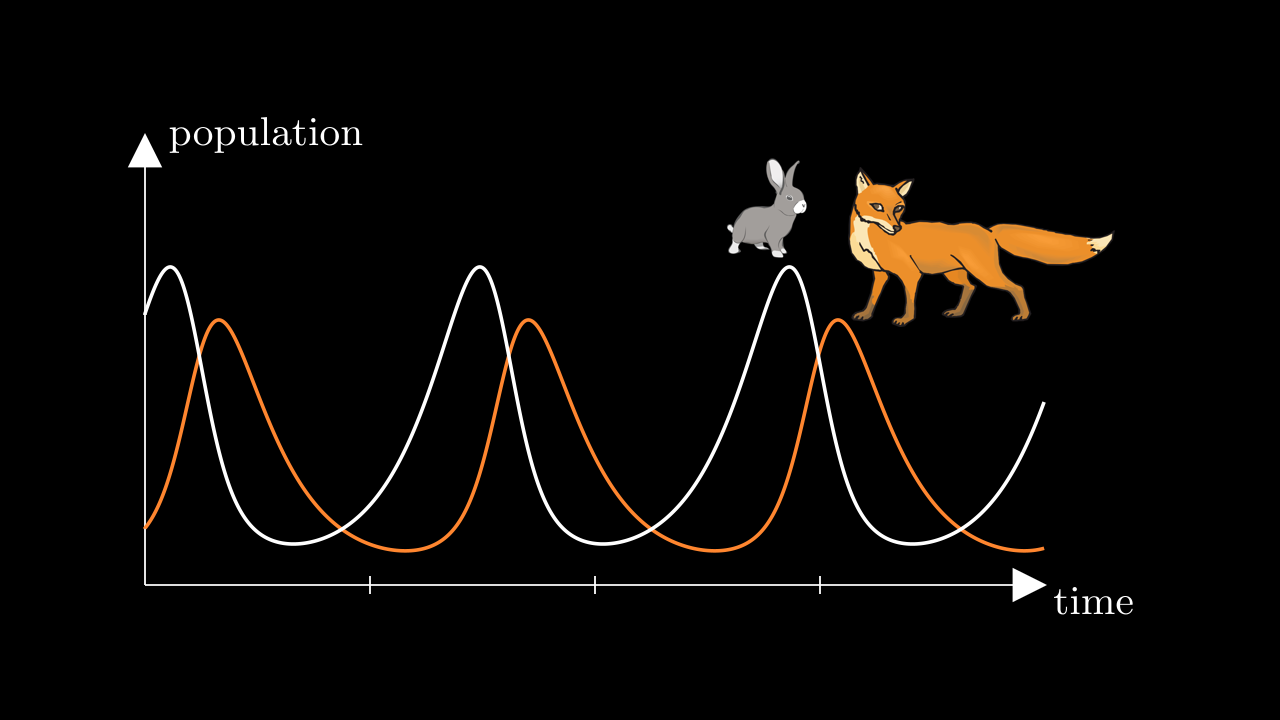
The populations fluctuate in a periodic way: after a certain amount of time, the population sizes are exactly what they were in the beginning. Then they repeat the same rise and fall over and over again.

The periodicity can be explained by the fact that the system has a conserved quantity

\[ F(x,y) = \alpha \log(y) – \beta y + \gamma \log(x) – \delta x \,. \]

“Conserved quantity” means exactly what it says on the tin: \( F(x,y) \) does not change over time. You can check that

\[ \frac{d F}{d t} = \frac{\partial F}{\partial x} \frac{d x}{d t} + \frac{\partial F}{\partial y} \frac{d y}{d t} \]

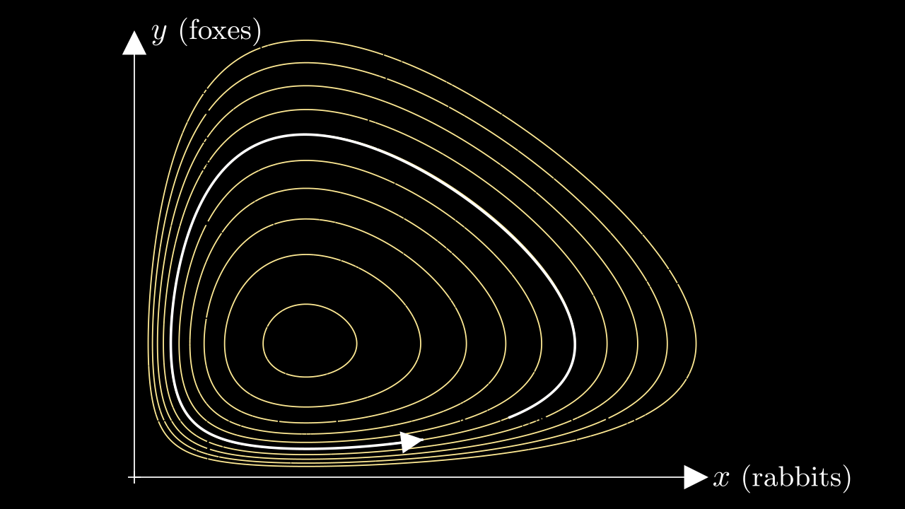
is zero by virtue of the Lotka-Volterra equations (1)-(2). We can also confirm this graphically by drawing a contour plot of \( F(x,y) \) and comparing it to the curve that a solution traces in the \( (x,y) \)-plane. We see that the solution stays on one of the level sets of \( F \):

The Volterra Chain

To keep our equations simple, let’s set all the constants equal to 1 and consider the system
\[ \begin{cases}
\displaystyle \frac{\mathrm d x}{\mathrm d t} = (1 – y) x \,, \\
\displaystyle \frac{\mathrm d y}{\mathrm d t} = (x – 1) y \,.
\end{cases} \]

What if we add another species to the ecosystem? One that eats foxes. If we denote its population size by \( z \), then the system of equations becomes

\[ \begin{cases}
\displaystyle \frac{\mathrm d x}{\mathrm d t} = (1 – y) x \,, \\
\displaystyle \frac{\mathrm d y}{\mathrm d t} = (x – z) y \,, \\
\displaystyle \frac{\mathrm d z}{\mathrm d t} = (y – 1) z \,.
\end{cases} \]

Now why stop at three? Consider a whole sequence of species \( q_1, \ldots, q_n  \), such that each species eats the species whose index is one less. This leads to the system of equations

\[ \begin{cases}
\displaystyle \frac{\mathrm d q_1}{\mathrm d t} = (1 – q_2) q_1 \,, \\
\displaystyle \frac{\mathrm d q_i}{\mathrm d t} = (q_{i-1} – q_{i+1}) q_i \qquad \text{ for } i = 2, \ldots, n-1 \,, \\
\displaystyle \frac{\mathrm d q_n}{\mathrm d t} = (q_{n-1} – 1) q_n \,.
\end{cases} \]

This system of equations is known as the Volterra chain. As a biological model, it probably isn’t very realistic. It assumes that there is a long food chain where each species exclusively eats the one just below it. But this isn’t a biology-off, it’s a math-off. And mathematically, the Volterra chain is an interesting object.

The Volterra Chain is a discrete analogue of certain wave equations, where the continuous space variable of a wave equation is replaced by the discrete sequence of species forming our food chain. If we take a large number of species \(n\), it is not hard to see the wavy nature of this system:

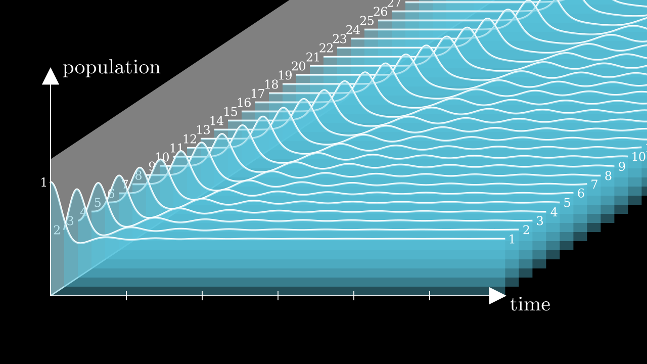
In this picture we started with a spike in population of species number 1, the lowest on the food chain. This perturbation ripples through the other species like a wave. After the wave has passed, population numbers settle back into the equilibrium.

Such a solitary wave, one that travels along without changing its shape, is called a soliton.

Solitons and water waves

There are several ways to approach the theory of soliton equations, but on some level they all come back to our observation that the two-species Lotka-Volterra model has a conserved quantity. Soliton equations have a lot of conserved quantities (infinitely many in fact). And it turns out that if you have an equation that conserves many different abstract things, you can deduce that it will also conserve some very tangible features, like the shape of a traveling wave.

Another equation that famously exhibits solitons is the Korteweg-de Vries (KdV) equation, modelling waves in a shallow canal. You can see an example of a KdV soliton in this video from the Scripps Institution of Oceanography:

The mathematical description of the solitons and other features of the KdV equation mimics that of the Volterra chain. In fact, you can consider the KdV equation as a limit of the Volterra chain with infinitely many species!

Mats Vermeeren is a Research Fellow and Lecturer at Loughborough University, UK. He is a Dutch-speaking Belgian. Dutch is one of the few languages in which the word for “maths” does not derive from the Greek “máthèma”, so his parents had no idea what they predestined him for. You can follow him on YouTube and Mathstodon, or look at his homepage.

Impress your friends by visualizing 1/3+1/9+1/27+1/81+… using any random book

Howie shows how you can physically show the sum of this infinite series with any book!

Howie Hua teaches math to future elementary school teachers at Fresno State. He also likes to make math explainer videos and math memes. You can find all his socials on his linktree.

So, which bit of maths has tickled your fancy the most? Vote now!

 Loading ...

The poll closes at 08:00 BST tomorrow. Whoever wins the most votes will get the chance to tell us about more fun maths in the quarter-final.

Come back tomorrow for our fifth match in round 1, pitting Matt Peperell against Fran Watson, or check out the announcement post for your follow-along wall chart!