Welcome to the eighteenth match in this year’s Big Math-Off. Take a look at the two interesting bits of maths below, and vote for your favourite.

You can still submit pitches, and anyone can enter: instructions are in the announcement post.

Here are today’s two pitches.

Matthew Scroggs – A surprising fact about quadrilaterals

Matthew Scroggs is one of the editors of Chalkdust, a magazine for the mathematically curious, and blogs at mscroggs.co.uk. He tweets at @mscroggs.

Recently, I came across a surprising fact: if you take any quadrilateral and join the midpoints of its sides, then you will form a parallelogram.

The first thing I thought when I read this was: “oooh, that’s neat.” The second thing I thought was: “why?” It’s not too difficult to show why this is true; you might like to pause here and try to work out why yourself before reading on…

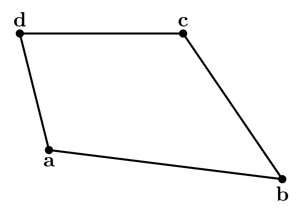
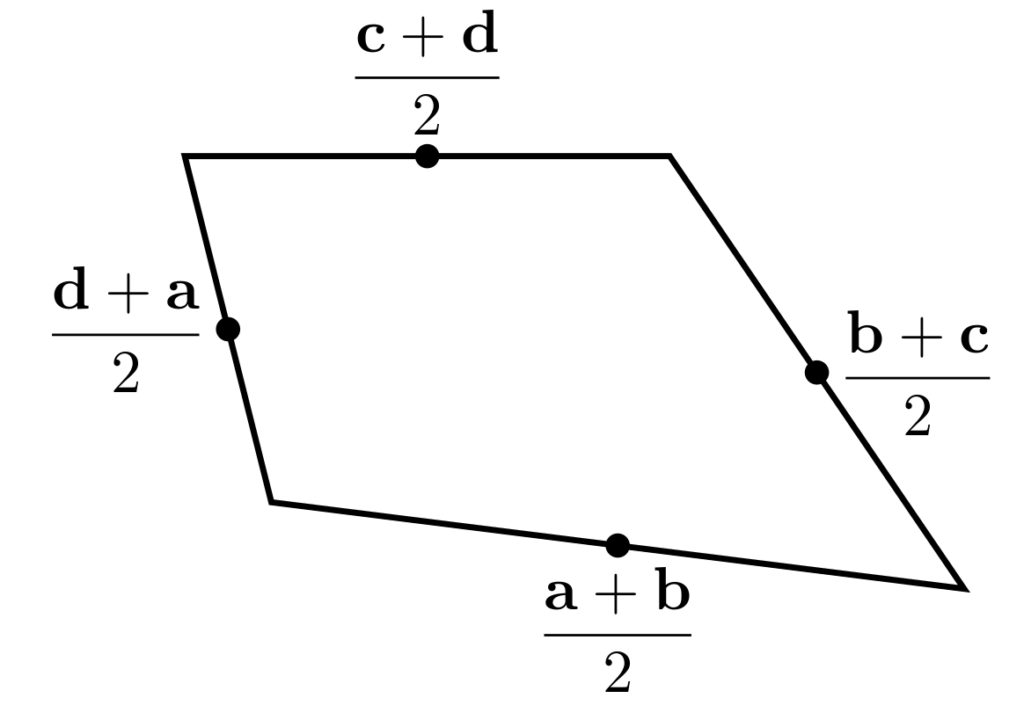
To show why this is true, I started by letting $\mathbf{a}$, $\mathbf{b}$, $\mathbf{c}$ and $\mathbf{d}$ be the position vectors of the vertices of our quadrilateral. The position vectors of the midpoints of the edges are the averages of the position vectors of the two ends of the edge, as shown below.

We want to show that the orange and blue vectors below are equal (as this is true of opposite sides of a parallelogram).

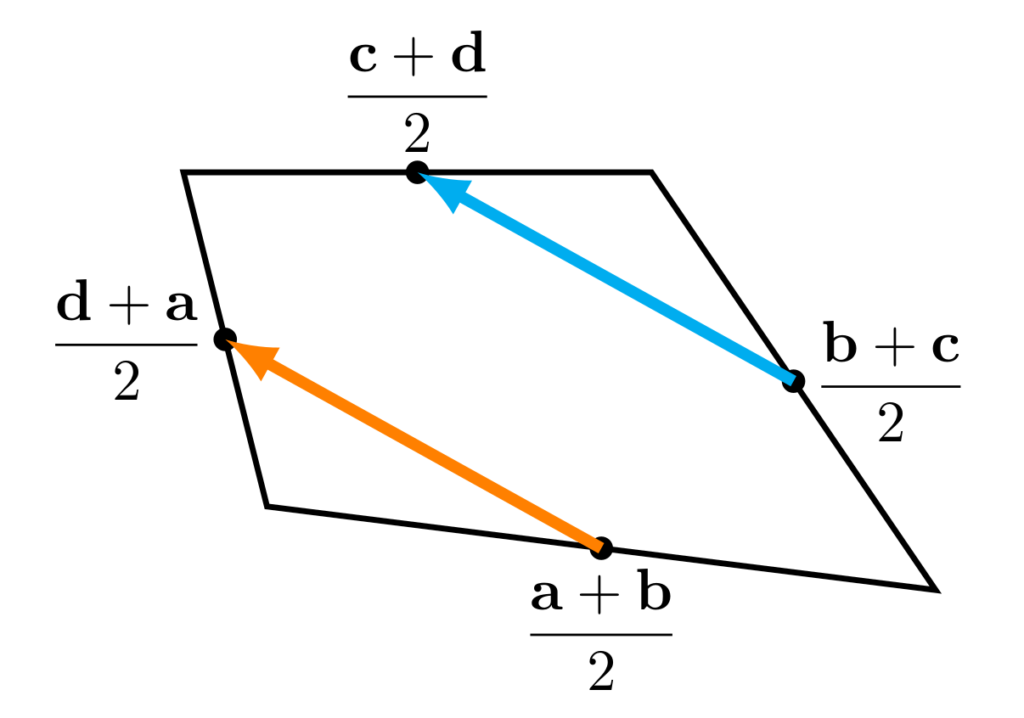
We can work these vectors out: the orange vector is
$$\frac{\mathbf{d}+\mathbf{a}}2-\frac{\mathbf{a}+\mathbf{b}}2=\frac{\mathbf{d}-\mathbf{b}}2,$$
and the blue vector is
$$\frac{\mathbf{c}+\mathbf{d}}2-\frac{\mathbf{b}+\mathbf{c}}2=\frac{\mathbf{d}-\mathbf{b}}2.$$

In the same way, we can show that the other two vectors that make up the inner quadrilateral are equal, and so the inner quadrilateral is a parallelogram.

Going backwards

Even though I now saw why the surprising fact was true, my wondering was not over. I started to think about going backwards.

It’s easy to see that if the outer quadrilateral is a square, then the inner quadrilateral will also be a square.

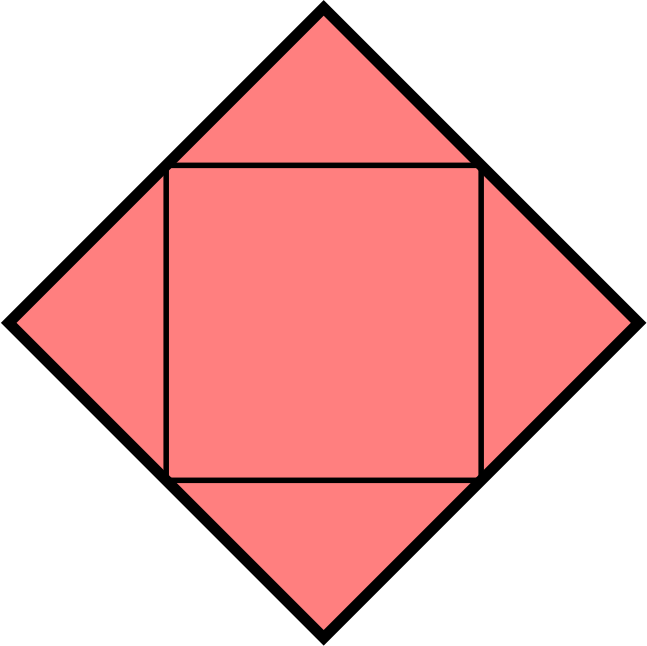
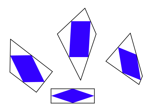
It’s less obvious if the reverse is true: if the inner quadrilateral is a square, must the outer quadrilateral also be a square? At first, I thought this felt likely to be true, but after a bit of playing around, I found that there are many non-square quadrilaterals whose inner quadrilaterals are squares. Here are a few:

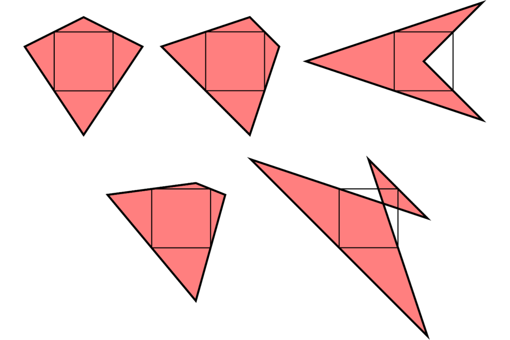
There are in fact infinitely many quadrilaterals whose inner quadrilataral is a square. You can explore them in this Geogebra applet by dragging around the blue point:

As you drag the point around, you may notice that you can’t get the outer quadrilateral to be a non-square rectangle (or even a non-square parallelogram). I’ll leave you to figure out why not…

Andrew Stacey – What’s the time, Mister Wolf?

Andrew Stacey writes about maths at loopspace.mathforge.org and tweets at @mathforge.

Knowing the right time can be a difficult task. At the moment, I’m having trouble remembering what day it is let alone the number of milliseconds that passed since midnight. Fortunately, computers can do these things without getting distracted. But even there the answer is not always completely obvious.

For a program I wrote recently I wanted to know the time very accurately. I was messing around with making a clock and wanted smooth transitions for the seconds counter, meaning that I needed to know the time more precisely than the nearest second.

There was a snag, however. The environment that I was using didn’t have a single clock that I could use. It had two clocks, neither of which did by itself what I wanted. One clock told me the time, but only to an accuracy of seconds. The other clock measured in milliseconds, but only told me the time elapsed from the start of the program.

Think of one as a normal clock where you can see the hours, minutes, and seconds but no more, and the other as a stopwatch that has been started at some random juncture.

My question was: How could I use these to tell the time?

Obviously, I wanted to take the hours, minutes, and seconds from the clock. Those were accurate – in fact, there is presumably a more accurate clock inside the device that I was programming which ensures that what this clock tells me is correct. It is the milliseconds that cause the difficulty.

Clearly, if I knew the value of one clock at a significant moment for the other then I could use that information to calculate the number of milliseconds in the current second. For example, if I knew the precise time – to the millisecond – that the program started then I could just use that together with the number of milliseconds since then to get the precise current time.

Or if I knew the number of milliseconds at which the clock ticks over from, say, $18:42:24$ to $18:42:25$ then I could use that marker to adjust the milliseconds to know the precise current time. If that happened, say, at $48134$ milliseconds since the program started then I know that the seconds tick over when the stopwatch reads some thousands and $134$ milliseconds, so I simply take the current millisecond reading, say $78341$, subtract $134$, $78341 – 134 = 78207$, then drop the thousands to result in the current millisecond reading, in this case of $207$.

This suggests a strategy: watch the clock and at the moment that the seconds change on the clock note the time on the stopwatch.

But there’s another snag. It’s as if I’m blinking when I look at these clocks so I don’t notice the exact moment that the seconds change. All I can do is notice that they’ve changed since the last time I looked. Admittedly, I’m “blinking” at about sixty times a second, but to get an accuracy of milliseconds then this isn’t fast enough.

It’s time (ha ha) to deploy Math.

Let $a$ denote the actual number of thousandths of a second when the clock clicks over from one second to the next. In the example above, we would have $a = 134$ (but in the program we don’t know what value this is). Every time the program blinks we note the time on the clock and the stopwatch. We are looking for a time when the seconds change on the clock. When this happens, we make special note of the time on the stopwatch and the previous reading on the stopwatch before the change. Let’s call these $b$ and $c$, with $b$ the previous reading and $c$ the current reading.

Now the actual time on the stopwatch when the clock ticked over will have been some thousands plus $a$. That is, there is some $d$ such that the time on the stopwatch was $1000d + a$. So we have the inequality:

\[ b \lt 1000d + a \le c \]

which we can rearrange to an inequality for $a$:

\[ b – 1000d \lt a \le c – 1000d\]

So when the clock ticks over we get an interval in which $a$ lies.

Every second, therefore, we get new information on where $a$ can be found. We keep a running record of our current “interval of knowledge” and when a new interval comes in then we intersect with the current interval to update it.

In the specific circumstance, our intervals are roughly $\frac{1}{60}$th of a second in width. If we assume that they are uniformly distributed, subject to the constraint that they contain $a$, then we can consider an interval of width $\frac{1}{60}$ to be determined by its lower limit which must lie in the interval $[a – \frac{1}{60}, a]$ so we can model this by a random variable uniform on that interval.

Then given a family of such $X_{i}$, our current “interval of knowledge” is found by intersecting all the intervals $[X_{i}, X_{i} + \frac{1}{60}]$. As we intersect these, the lower bound is the maximum of the lower bounds of these intervals and the upper bound is the minimum of their upper bounds. So our interval of knowledge is:

\[ \left [ \max (X_{i}), \min (X_{i}) + \frac{1}{60} \right ] \]

Its width is therefore modelled by:

\[\min (X_{i}) + \frac{1}{60} – \max (X_{i}) = \frac{1}{60} – (\max (X_{i}) – \min (X_{i})) \]

Now life is always easier if we standardise to $[0,1]$. So let us assume that $Y_{i}$ is uniform on $[0,1]$. The distribution of $\max (Y_{i})$ is $n y^{n-1}$ where $n$ is the number of readings. This comes from differentiating the cumulative distribution, starting from the fact that:

\[ P(\max (Y_{i}) \le y) = \prod P(Y_{i} \le y) = y^{n} \]

So the expected value of $\max (Y_{i})$ is:

\[ \int_{0}^{1} y n y^{n-1} d y = n \int_{0}^{1} y^{n} d y = \frac{n}{n+1} \]

and of $\min (Y_{i})$ is $1 – \frac{n}{n+1} = \frac{1}{n+1}$. Therefore, the expected value of $\min (Y_{i}) – \max (Y_{i}) + 1$ is

\[ \frac{1}{n+1} – \frac{n}{n+1} + 1 = \frac{1 – n + n+1}{n+1} = \frac{2}{n+1} \]

Rescaling to the $X_{i}$ simply means multiplying by $\frac{1}{60}$.

So we expect that our ignorance about $a$ to be approximately $\frac{1}{30(n+1)}$ after $n$ seconds. Since we’re reading milliseconds, we should have a good idea of $a$ when $30(n+1) \gt 1000$, or $n \gt 33$.

After half a minute, then, we should have a good idea as to where $a$ actually lies and we should then be able to get a fully accurate time, including milliseconds.

Of course, there are implementation issues. What should we do before we know $a$ accurately? And if we update our knowledge and so refine our estimate of $a$, do we change in a snap or should we change gradually? There’s also an issue of how to correctly convert our readings of $b$ and $c$ into the interval for $a$ since we have to subtract $1000d$ but don’t know what $d$ is. But these are mere technicalities.

By combining our knowledge, we’ve upgraded our seconds-accurate clock and milliseconds-accurate stopwatch to a milliseconds-accurate clock. So I can make my fancy display clock have nice transitions between the seconds.

So, which bit of maths made you say “Aha!” the loudest? Vote:

 Loading ...

The poll closes at 9am BST on Sunday the 17th, when the next match starts.

If you’ve been inspired to share your own bit of maths, look at the announcement post for how to send it in. The Big Lockdown Math-Off will keep running until we run out of pitches or we’re allowed outside again, whichever comes first.