Welcome to the twenty-third match in this year’s Big Math-Off. Take a look at the two interesting bits of maths below, and vote for your favourite.

You can still submit pitches, and anyone can enter: instructions are in the announcement post.

Here are today’s two pitches.

Karen Campe – Easy Angles

Karen Campe is a mathematics teacher, teacher educator, and math technology consultant from Connecticut. You can find her on Twitter at @KarenCampe.

Many of us are stuck at home these days; what if you need to measure angles and just don’t have a protractor? You can quickly distinguish acute and obtuse angles with one of the right angles you carry around all the time – the angle formed by your thumb and index finger – but that is hardly a precise instrument for measuring! In this pitch, I will share with you some easy angle tools that you can create with only a piece of paper.

Right angles and 45°

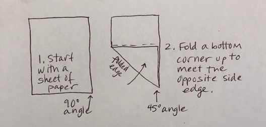
The corner of a sheet of paper is a more exact right angle than that created by our fingers, and I have suggested this to my students when they are first learning to visualize acute angles that are smaller than 90° versus obtuse angles that are bigger.

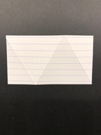
To create an easy 45° angle, fold a sheet of paper diagonally so one edge aligns with the adjacent edge, bisecting the right angle:

Now you can measure 90° and 45° angles, as well as determine whether your angle is larger than 90°, smaller than 45°, or between those values. For more precision, fold your folded edge to meet the same side edge as before, and this bisection of the 45° creates 22.5° and 67.5° demarcations as well.

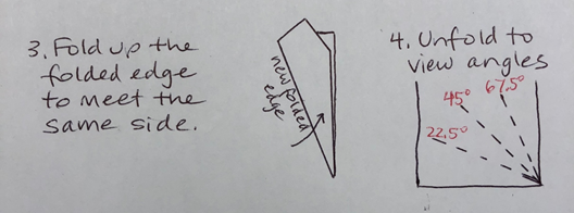
This bisecting strategy works, but the angle sizes created aren’t especially useful (except for defining the intervals). Let’s create some commonly used angles next.

More Useful Angles

After 45° and 90°, arguably the most mathematically useful angle sizes are 30° and 60°.

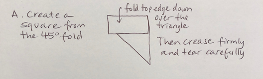
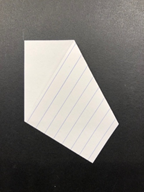
A. Begin with a square piece of paper – create this by doing steps 1 and 2 above, and then cutting off the rectangle section at the top. No scissors? Simply fold the top edge down over the triangle, press your finger along the fold, reverse the fold and press firmly again, then tear carefully along the crease line.

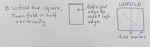
B. Unfold the square, then fold the paper in half vertically: fold the right edge over to the left edge to make a crisp vertical crease down the middle of the square. Unfold again.

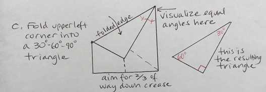
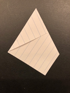
C. Fold the upper left corner into a triangle, by folding it down towards the lower part of the vertical crease.
• Aim that corner approximately 2/3 of the way down the vertical crease
• Visualize the angles being created in the upper right of your paper – the folded-over piece should look equal to the visible portion of the underneath paper.
• You have created a triangle that has angles measuring 30°, 60°, and 90°.
Can you explain why the 30° angle has that measure?

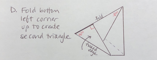
D. Fold the bottom left corner up to form a second triangle. Fold until the left edge of the paper lines up with the creased edge of the first triangle.
• This is also a 30°-60°-90° triangle. You can check the 60° angle is the same size as the one in the layer below that was formed in step C, and if you unfold all the way, it is clear that 3 equal angles equal 180° because they make the straight edge of the paper.

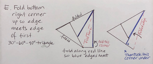
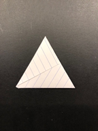
E. Fold the bottom right corner up, so the right edge of the paper meets the edge of the first 30°-60°-90°. Then tuck the corner under the second 30°-60°-90° triangle.

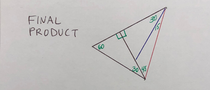
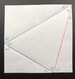
F. The Final Product is a 45°-60°-75° triangle! The 15° angle was created by bisecting a 30° angle, and the 75° (30° + 45°) is its complement. Use this “protractor” to measure these special angles, and estimate the size of angles that fall between measurements. Ask students to unfold and label other angles.

A Business Card Special Triangle?

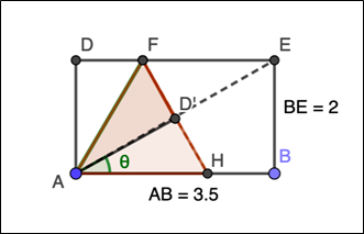
Take a standard US business card, which measures 3.5 inches by 2 inches, and fold the upper right corner down to meet the lower left corner. Next fold the upper left corner over to meet the folded edge, and finally, the corner that is pointing down folds underneath the rest. What is the result? Can you see the equilateral triangle and the 30°-60°-90° triangle?

It’s a great cocktail party trick, but is it actually an equilateral triangle? Here is the construction; the angle marked $\theta$ is half of one of the triangle’s angles. Does it equal 30° as expected for half an angle in an equilateral triangle? Sadly, no, the inverse tangent of $2 \div 3.5 \approx 29.74^\circ$. Close enough to visualize, but not exact! Check out the GeoGebra visualization.

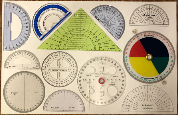
I hope you’ve enjoyed this pitch about folding your own protractor from paper. And if you really need a protractor to borrow, I’ve got plenty!

Tom Briggs – Venus Transits and the Size of the Solar System

Tom Briggs is a maths educator working in the Heritage sector, and tweets as @TeaKayB

In the early 1600s Johannes Kepler published his laws of planetary motion, discovered through analysis of detailed observations made by Tycho Brahe. The third of these laws is:

The square of the orbital period of a planet is directly proportional to the cube of the semi-major axis of its orbit.

More succinctly: $R^3=kT^2$, where $R$ is the semi-major axis of a planet’s orbit, $T$ is the time taken for it to complete one orbit, and $k$ is an unknown constant.

Without $k$, Kepler’s third law made it possible to find relative distances for any planet with decent observational data: if we say that Earth’s orbital period is $1$ (that’s kind of the definition of a year) and that its average orbital radius is $1$ (that’s kind of the definition for an Astronomical Unit), then $k = 1$.

For Jupiter, the orbital period ($T_J$) is known (about 11.86 Earth years), so the average orbital radius ($R_J$) is:

\begin{align}
R^3_J &= T^2_J \\
&= 11.86^2 \\
R_J &= \sqrt[3]{11.86^2} \\
&\approx 5.2
\end{align}

The units are “average orbital radii of Earth” which is a bit of a mouthful so it’s easier to call it $R_E$. That means that given the data available to Kepler and his insight into the relationship between orbital periods and radii we can work out that Jupiter is about 5 times further from the Sun than Earth is (or, $5R_E$), but we still don’t know any actual distances.

We can do the same thing for all planets, so we could draw accurate maps of the entire (known) Solar system with one key omission: a scale. Finding just one distance would allow the rest to slot into place.

Around a hundred years later, Edmund Halley (yes, the one named after the Comet) proposed a method (Building on suggestions by James Gregory in 1663) for using solar transits of Venus to fill in the gap.

A “solar transit” is when something passes in front of the Sun according to a viewer. Solar transits of Venus as viewed from Earth happen in pairs about 8 years apart, repeating every 243 years. The last pair were in 2004 & 2012.

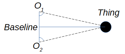
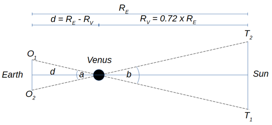
Halley’s idea began with triangulation, which was not new. Figure 1 shows the setup: Two observers ($O_1$ & $O_2$) measure the distance between themselves (the baseline) and the angle between this baseline and a distant object. In the simplest situation (an isosceles triangle, as in Figure 1) it’s a matter of basic trigonometry to find the distance from the baseline to the thing.

When observers are based far apart on the curved surface of the Earth, however, the baseline is an imaginary line passing through the Earth itself. Calculating the length of this line is easy enough if you can find your longitude (Working out how to work that out is easily another entry’s worth of stuff…) to a decent accuracy, but there’s nothing tangible from which to measure the angles to the thing (in our case, Venus). If you could just find the third angle (angle $a$, Figure 2) you’d be cooking on gas .

This is where the idea of parallax comes in.

Simply put, parallax is that thing where you close one eye, hold your thumb up to cover a picture on the wall, then swap eyes so that your thumb is covering a different picture. It’s what makes nearby lampposts rush past the car much faster than more distant trees.

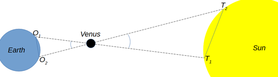
In the context of this post, Venus is the thumb, the Sun takes the place of the wall, and $O_1$ & $O_2$ play the part of your eyes. In Figure 2, $T_1$ is the bit of the Sun covered up by Venus as far as $O_1$ is concerned, and $T_2$ is the equivalent point from $O_2$’s viewpoint.

The problem here is that the Sun is relatively featureless so it’s very difficult to record exactly which bit is covered by Venus. Also, synchronising measurements is pretty hard when you’re hundreds of miles apart.

Halley’s idea was for each observer to record the time taken for Venus to transit the Sun from start to finish. In Figure 3, you can see that the setup isn’t quite so neat as Figures 1 & 2 suggested. This means that Venus appears to cross different parts of the Sun’s disk from each observation point (the difference is massively exaggerated here), Figure 4 shows two (similarly exaggerated) trails across the Sun, as recorded by $O_1$ and $O_2$ respectively.

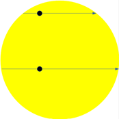
Venus is moving at the same speed for both observers, but the transit paths are different lengths (It’s quite important, though beyond the scope of this post to discuss at length, that the two paths are parallel.) (see Figure 4), which means the time recorded for each transit is different. This difference allows a relatively accurate determination of the apparent “distance” between the paths. “Distance” is in inverted commas here because it is an angular distance which means that it is actually an angle. The angle in question is the one formed by the crossing of the lines-of-sight from $O_1$ to $T_1$ and from $O_2$ to $T_2$ (angle $b$, Figure 3).

Things now fall into place fairly quickly… Angle $a$ is identical to angle $b$, which means we can work out the distance from Earth to Venus ($d$) using this, the length of the baseline, and some trigonometry. From Kepler’s 3rd law we know that Venus’ orbit is 0.72 times the size of Earth’s, so given that:

$d=R_E-R_V$ and $R_V=0.72\times R_E$

then:

\[ R_E=\frac{d}{0.28} \]

This relatively simple idea was a major stepping stone in our exploration of the cosmos, increasing our understanding of the sheer scale of the universe that surrounded us, and allowing us to start properly mapping our place within it.

Further thinking:

1. The model above is heavily simplified. What are the complications?
2. More accurate methods have since been used to verify the 18th Century calculations of the Earth-Sun distance and have found them to be within around 2% of modern values. What might these modern methods be?
3. A cracking read about the 1761 and 1769 expeditions to observe the Venus transits for exactly this purpose is Chasing Venus by Andrea Wulf. Be warned, however, that it doesn’t contain much maths.

So, which bit of maths made you say “Aha!” the loudest? Vote:

 Loading ...

The poll closes at 9am BST on Thursday the 28th, when the next match starts.

If you’ve been inspired to share your own bit of maths, look at the announcement post for how to send it in. The Big Lockdown Math-Off will keep running until we run out of pitches or we’re allowed outside again, whichever comes first.