Here’s the seventh match in Round 1 of The Big Internet Math-Off. Today, we’re pitting Fran Herr against Tom Edgar.

Take a look at both pitches, vote for the bit of maths that made you do the loudest “Aha!”, and if you know any more cool facts about either of the topics presented here, please write a comment below!

Fran Herr – Modular Multiplication and Dancing Planets

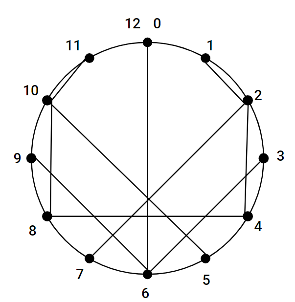
This is a story about fantastical patterns emerging from a pair of integers, and it has more to do with geometry than number theory (*sighs with relief*). Start with a positive integer \(m\) and place \(m\) evenly spaced points around a circle, labeling them \(0, 1, \dots, m -1\). Then choose another integer \(a\) to be the multiplier. For each point labeled \(p\), draw a chord of the circle connecting \(p\) and \(ap \bmod m\). The resulting arrangement of chords is our main object of study; we will call it a modular multiplication table and denote it \(\mathop{\mathrm{MMT}}(m,a)\).

You may know these pictures by another name: “string art,” “light caustics,” “spirographs,” or “curve stitching,” for example. They are popular across the math communication world. The following question has been partially answered, but today we dive deeper than you have likely been before!

Given the values for \(m\) and \(a\), what pattern will \(\mathop{\mathrm{MMT}}(m,a)\) create?

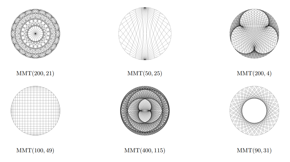
From the small selection of modular multiplication tables below, one can see that they are an eclectic bunch.

I encourage you to draw some of these tables for yourself as you read! There are many tools to do so online (made by people who know how to make webapps); one that I like is this one. You can also download my python code or write a quick script yourself.

We see our first pattern by fixing \(a\) at a “small” value and increasing \(m\); as we do this, a well-known curve emerges. For example, the picture below shows this process for \(a = 2\) and we see everyone’s favorite plane curve: the LOVEly cardioid <3.

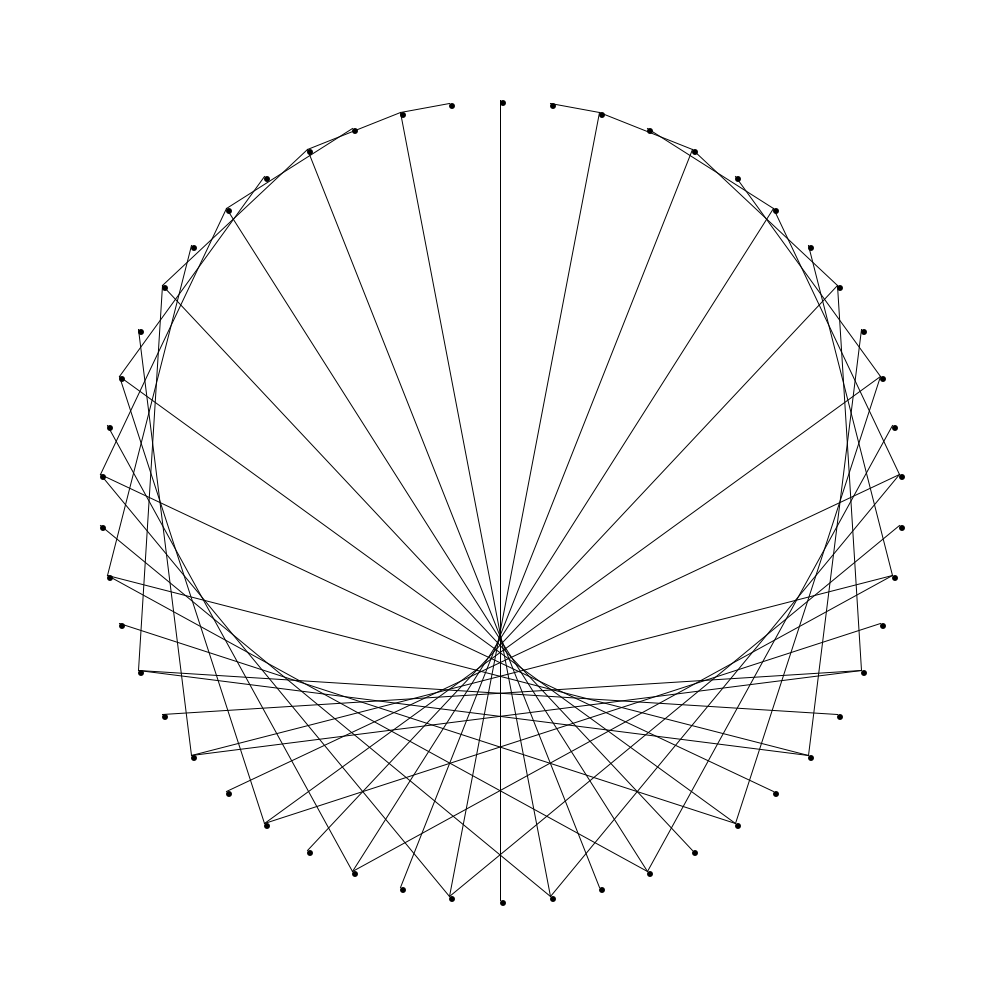
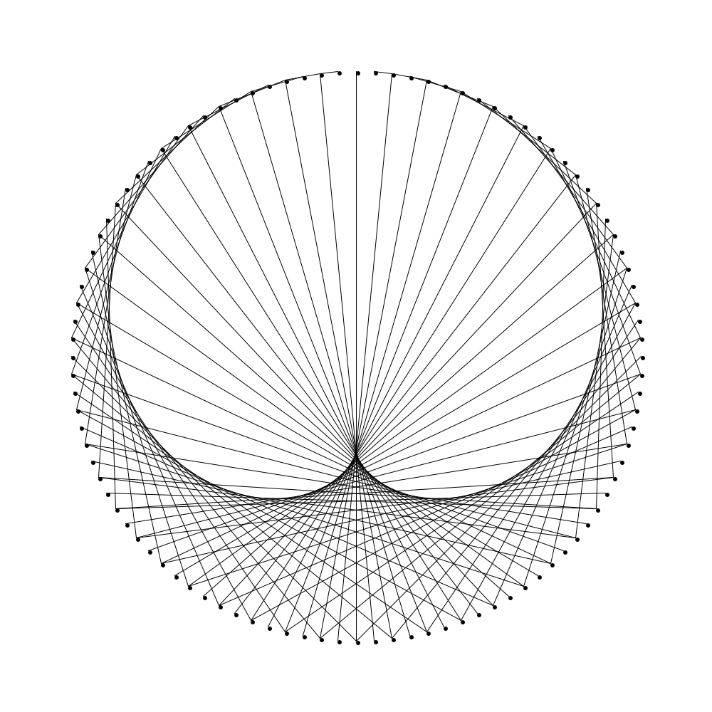
This curve, to which all the chords are tangent, is called the envelope of the chords. As we repeat this experiment with \(a = 3, 4, 5,\dots\) we notice a pattern.

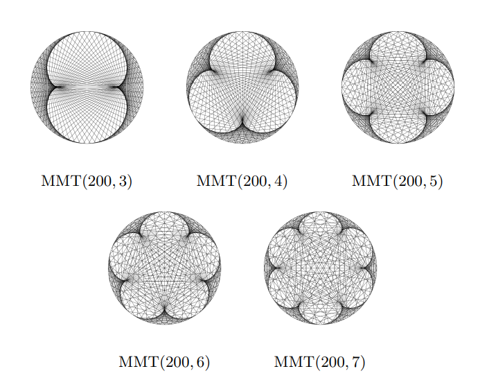
These curves are called epicycloids. The epicycloid with \(a – 1\) humps is made by rolling a circle with radius \(\frac{1}{a+1}\) around a fixed circle with radius \(\frac{a-1}{a+1}\) and tracking a point on the boundary of the outer circle. These curves are not the main focus for today, but they are neat and you can learn more about them from the wikipedia page. As we experiment with small values of \(a\) (between \(a=2\) and \(a = 12\) approximately), we might be led to believe that the envelope of \(\mathop{\mathrm{MMT}}(m,a)\), for sufficiently large \(m\), is always the epicycloid with \(a – 1\) humps. But in fact, this is a hasty conclusion.

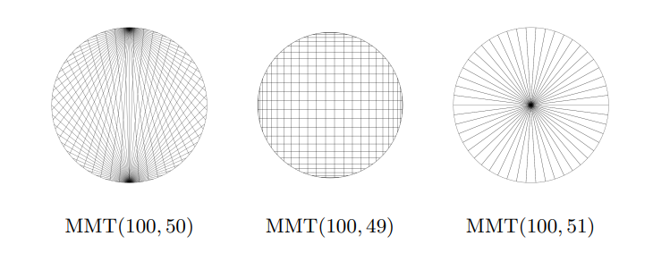
When we look at higher multipliers, we see the large variety of patterns showcased earlier. We notice that the numerical relationship between \(m\) and \(a\) plays a key role in determining the pattern. For example, tables of the form \(\mathop{\mathrm{MMT}}(2a, a)\) have a common shape independent of the choice for \(a\). A similar phenomenon happens for tables of the form \(\mathop{\mathrm{MMT}}(2a – 2, a)\), and \(\mathop{\mathrm{MMT}}(2a + 2, a)\).

Of course, you should not take me at my word! I encourage you to check by drawing more tables from the three families above. Bonus: Can you explain why we get these three patterns?

Another way to write these three families is to assume \(m\) is even and express them by

\[\mathop{\mathrm{MMT}}\left(m,\tfrac{m}{2}\right), \hspace{20pt} \mathop{\mathrm{MMT}}\left(m,\tfrac{m}{2} + 1\right), \hspace{10pt} \text{and} \hspace{10pt} \mathop{\mathrm{MMT}}\left(m, \tfrac{m}{2} – 1\right).\]

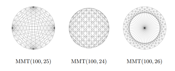
A natural generalization is to replace ‘2’ by an arbitrary ‘\(b\)’: assume \(m\) is divisible by positive integer \(0 < b < m\) and consider tables of the form

\[\mathop{\mathrm{MMT}}\left(m, \tfrac{m}{b}\right), \hspace{20pt} \mathop{\mathrm{MMT}}\left(m,
\tfrac{m}{b} + 1\right), \hspace{10pt} \text{and} \hspace{10pt} \mathop{\mathrm{MMT}}\left(m, \tfrac{m}{b} – 1\right).\]

The resulting designs for \(b = 4\) are shown below.

There are some beautiful patterns to understand here, and I encourage you to run some experiments yourself. But here we press forward. A few years ago, I became obsessed with modular multiplication tables and I went down this same line of exploration. The next question I asked was, “what if I dropped the assumption that \(b\) must divide \(m\)?” In this case we would still like to keep \(a\) as an integer, and so (for the first family) there are two natural choices for the multiplier:

\[\mathop{\mathrm{MMT}}\left(m, \left\lceil \frac{m}{b} \right\rceil\right) \hspace{10pt} \text{and} \hspace{10pt} \mathop{\mathrm{MMT}}\left(m, \left\lfloor \frac{m}{b} \right\rfloor\right).\]

Also, for each \(b\), there are \(b-1\) categories for \(m\) given by its equivalence class modulo \(b\). These families of tables display some amazing designs.

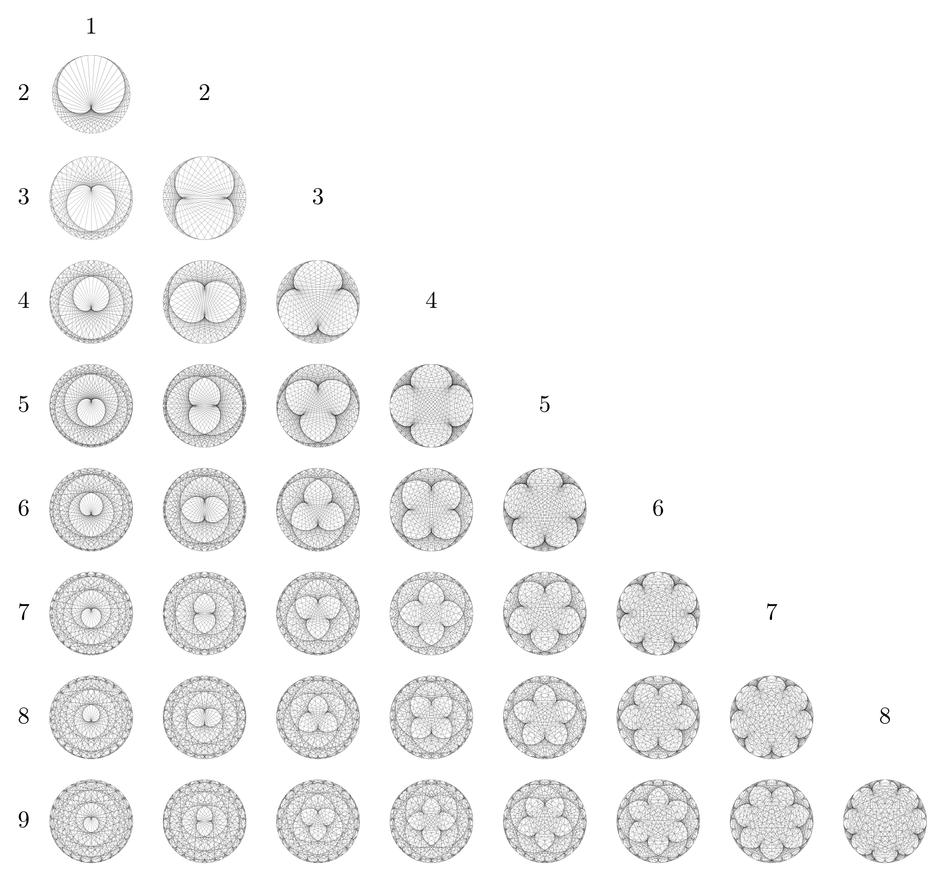
Figure 1 is a “table of tables”. Each table is of the form \(\mathop{\mathrm{MMT}}(m, \lceil \frac{m}{b}
\rceil)\) for some positive integers with \(b < m\). The rows are indexed by the value for \(b\) and the columns are indexed by \(r\) where \(m \equiv r \mod b\). We have taken \(m\) to be relatively large so as to see the pattern clearly. Most values for \(m\) are approximately \(200\).

I encourage you to pause and ponder this array. What patterns do you notice? Do the designs remind you of other curves we have looked at? Why do you think these patterns might be emerging?

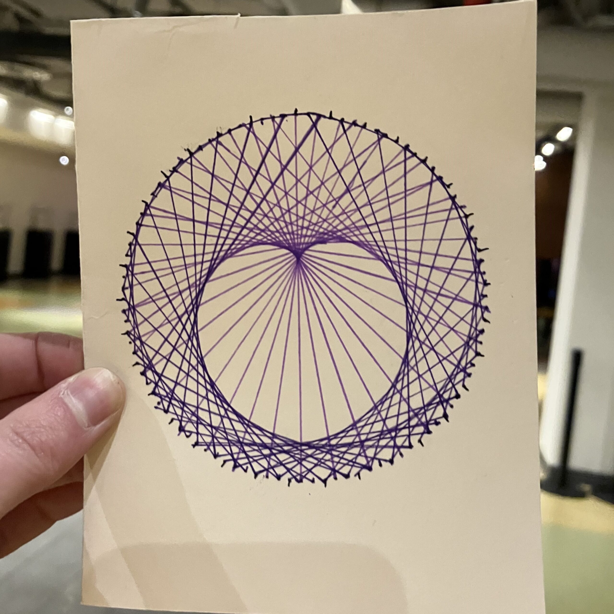
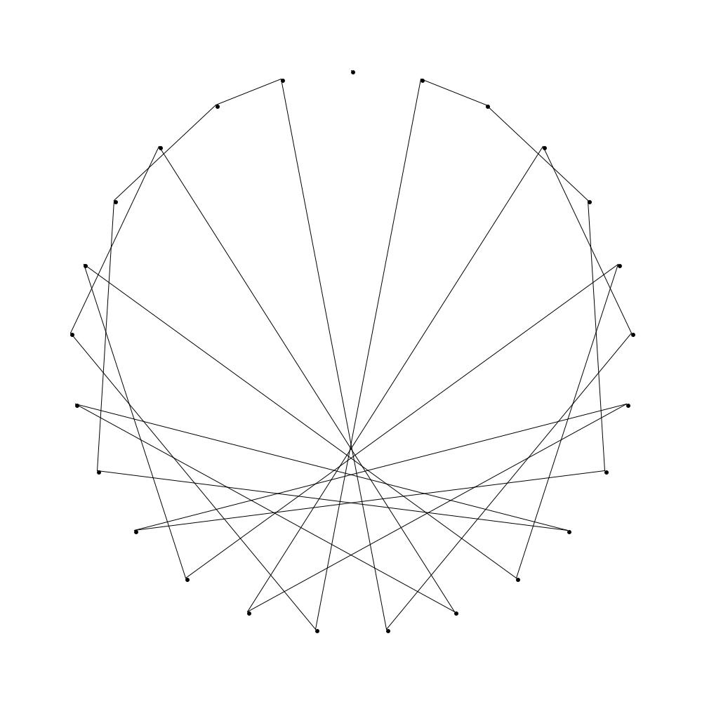
Let’s look at one particular example from this collection. The table \(\mathop{\mathrm{MMT}}(100,34)\) satisfies \(m \equiv 1 \mod 3\) and \(a = \lceil \frac{m}{3} \rceil\). Last year, I decided to draw this on a Valentine’s day card (seemed appropriate). I started by connecting 1 to 34, 2 to 68, and so on… but I soon noticed a pattern in the way the chords developed.

As we plot the chords one at a time, we notice that we can form the same pattern by moving the initial endpoint of the chord 3 spaces and the terminal endpoint 2 spaces. This observation unlocks a new perspective on these modular multiplication tables.

Imagine two planets, named A and B, on the same circular orbit around a central sun. Suppose an infinitely stretchy tether connects the two planets. At any one moment this forms a chord of their circular orbit. This setup is very similar to an animation by Matt Henderson, posted on Twitter, except in our case both planets are on the same orbit. We will call this system a planet dance.

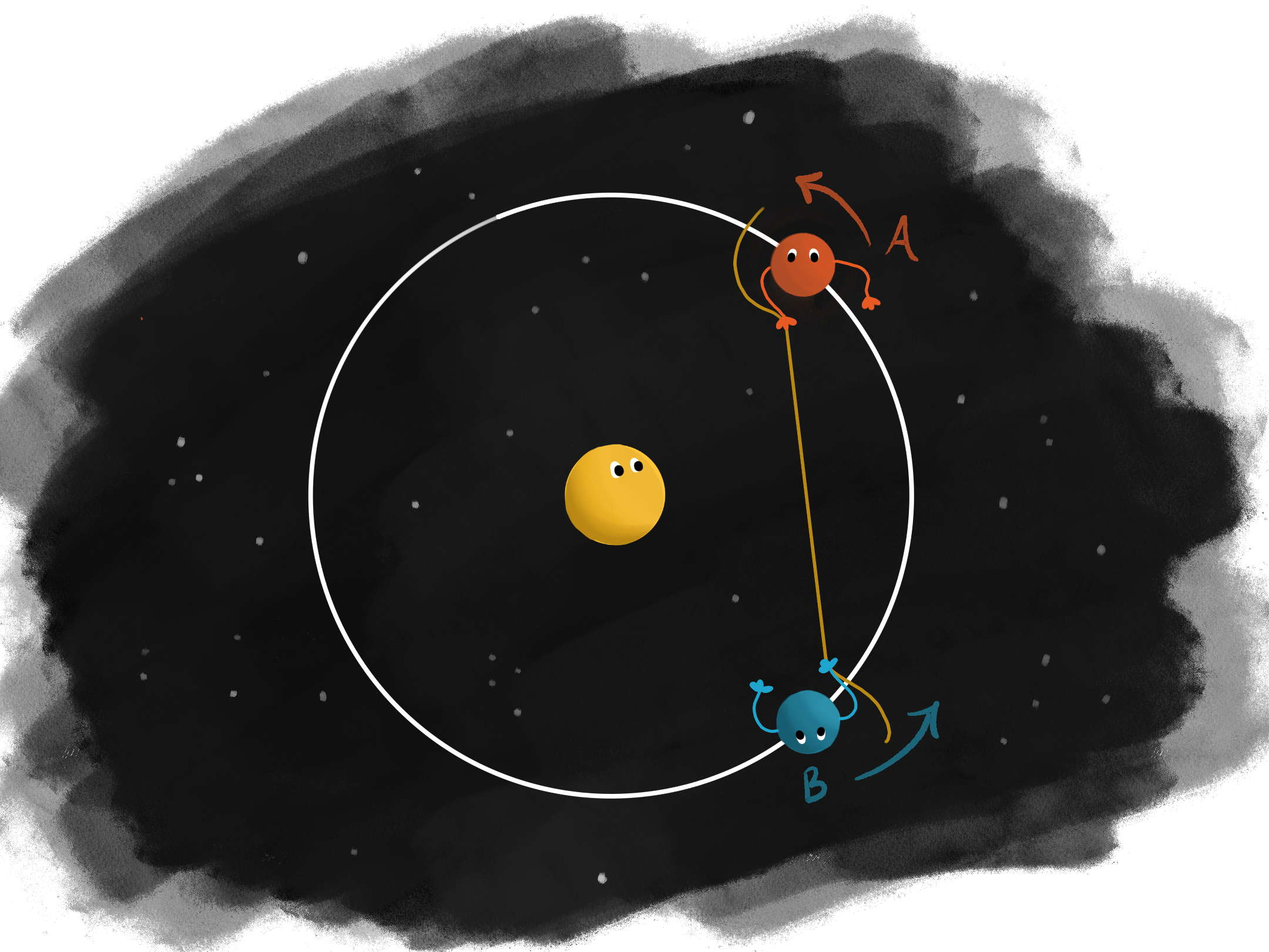
Formally, a planet dance, denoted by \(\mathcal{P}(\alpha, \beta)\) is defined by two integers \(\alpha\) and \(\beta\). It consists of the set of directed chords of the unit circle with initial point \(e^{2\pi i \alpha t}\) and terminal point \(e^{2\pi i \beta t}\), for all \(t \in [0, 1]\).

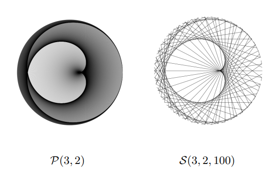
We can realize a modular multiplication table \(\mathop{\mathrm{MMT}}(m,a)\) as a discrete sampling of a planet dance. Set planet B orbiting \(a\) times faster than planet A, take a picture of the system at \(m\) regular intervals along planet A’s orbit, and overlay all these images. This is called an \(m\)-sampling of a planet dance \(\mathcal{P}(\alpha, \beta)\) and it is defined as a finite subset of \(\mathcal{P}(\alpha, \beta)\); those chords for which \(t = \frac{k}{m}\) for integer \(k\) with \(0 \leq k \leq m-1\). We denote this sampling by \(\mathcal{S}(\alpha, \beta, m)\).

Planet dances open up a whole new world; we can choose \(\alpha\) and \(\beta\) so that \(\frac{\beta}{\alpha}\) is not necessarily an integer. I again encourage you to graph these and look for patterns. You can do so again with my code or you can see the envelope of the curve by graphing the epicycloid in desmos.

Our observations above indicate that \(\mathcal{S}(1, 34, 100)\) and \(\mathcal{S}(2, 3, 100)\) actually produce the same set of chords. But why is that?

Now, finally, we can enter into topology land! A directed chord on the circle is uniquely determined by the position of the two endpoints, planet A and planet B. Hence, the space of all such possible chords is a circle times a circle: \(\mathbb S^1 \times \mathbb S^1 = T^2\)… a torus! So each point on the torus corresponds to a directed chord of the circle, and a planet dance is a continuous set of directed chords forming a linear path on the torus.

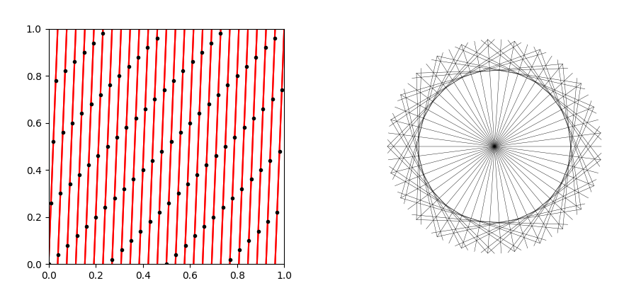
We model our torus as the unit square in \(\mathbb R^2\) with the opposite edges identified. We can think of this as the quotient space \(\mathbb R^2 / \mathbb Z^2\) where we identify points \((x,y) \sim (x + 1, y) \sim (x, y + 1)\). In this model, \(\mathcal{P}(\alpha, \beta)\) is given by the line \(\alpha y = \beta x\) in \(\mathbb R^2\) under this quotient map. This looks like a set of parallel diagonal line segments on the unit square.

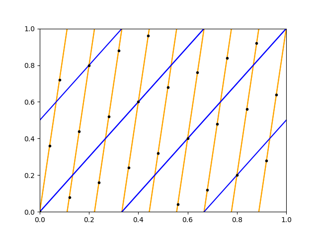
When we graph our two favorite planet dances (\(\mathcal{P}(1, 34)\) and \(\mathcal{P}(3, 2)\)), we see that they intersect exactly 100 times on the torus, and that these intersection points are at regular intervals because everything is linear. So when we sample either dance at a rate of 100, we get the same set of chords. And now, the mysteries begin to unravel.

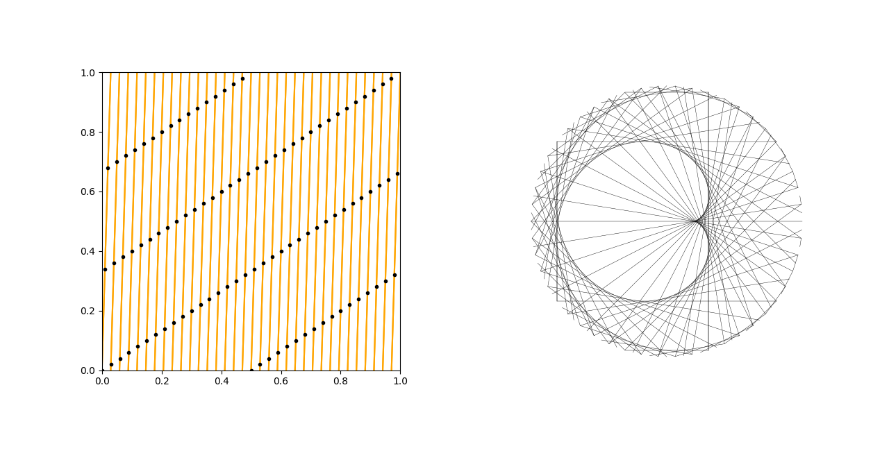
For a modular multiplication table \(\mathop{\mathrm{MMT}}(m,a)\), we can graph the sampling points of \(\mathcal{S}(1, a, m)\) on the unit square, and this reveals which planet dance is really the envelope of the curve: just connect the dots in the way that feel more “natural”. In our example above, we see that the black sampling points are positioned to trace out the line \(y = \frac{2}{3}x\) more naturally than \(y = 34x\).

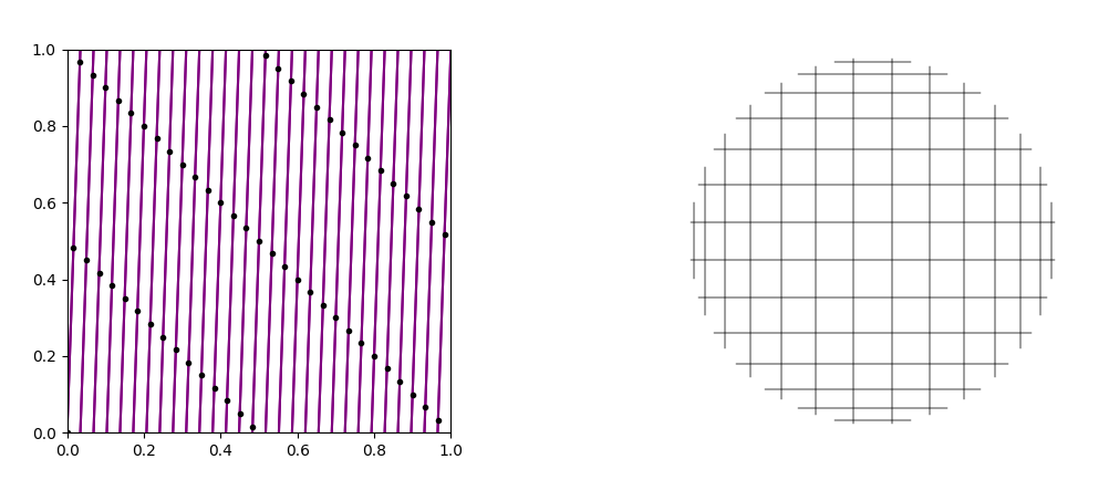
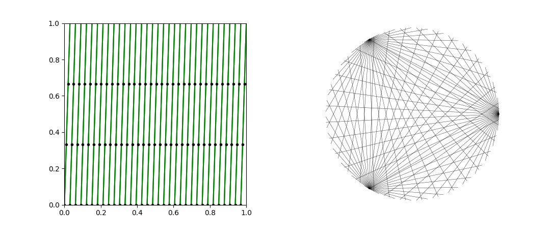
This phenomenon is a visual example of aliasing, a well-studied aspect of signal processing (hello applied mathematicians!). The \(\mathcal{P}(1, a)\) planet dance is undersampled as an MMT, and it ends up looking like a different planet dance. There is a lot more to uncover here! If you would like to read more about these ideas, I’ve written a full paper on it. But to end, I leave you with some more pictures of MMT’s and the corresponding sampled linear loops.

Fran Herr is a PhD student in mathematics at the University of Chicago. She studies low dimensional topology and geometric group theory. You can follow her on YouTube and X.

Tom Edgar – A Rational Day at the Hilbert Hotel

I want to tell you about a curious conundrum I encountered during my time working at the Hilbert Hotel. Maybe you’ve heard about the standard problem from the mystical lodge before, but in case not, here’s a quick recap of the classical story. The Hilbert Hotel contains infinitely many rooms, one for each natural number \(0,1,2,3,\ldots \). As legend goes, one night the hotel was full when a new traveler arrived and requested a room. The savvy hotel manager simply asked everyone currently staying in the hotel to move to the next room, thus opening room 0 for the new traveler. A similar strategy works if any finite number, say \(n\), of new travelers need rooms: simply repeat the process \(n\) times. Even more striking, if an infinite number of people (one for each natural number) need a room in the filled hotel, the hotel can accommodate them by simply sending the guest in room \(m\) to room \(2m\), thus opening all the odd rooms (see the video for an animation of the two different scenarios).

The classic Hilbert Hotel dilemma helps us learn to make sense of one-to-one correspondences between infinite sets. The last scenario succeeds because the set of natural numbers \(\{ 0,1,2,\ldots \} \) is in one-to-one correspondence with the set of even natural numbers \(\{ 0,2,4,6,\ldots \} \) via the map \(m\mapsto 2m\) and the set of odd natural numbers \(\{ 1,3,5,\ldots \} \) via the map \(m\mapsto 2m+1.\) The existence of these two correspondences allows the infinitely full hotel to make room for the infinitely many new guests.

I expected working at the hotel to be an easy gig because I thought I knew all the necessary tricks. But the job tested me immediately. On the first day after the hotel had been closed for renovations, an infinite collection of people, one for each positive rational number, requested a room. The positive rational numbers are numbers that can be written in the form \(p/q\) where \(p\) and \(q\) are both positive natural numbers. I wasn’t worried because I knew there is a one-to-one correspondence between the natural numbers and the positive rationals. Figure 1 distills the short form of the proof.

Figure 1: There exists a one-to-one correspondence between the natural numbers and the positive rationals (or more precisely pairs of positive natural numbers) since we can traverse anti-diagonals in order and eventually count to every rational.

The idea is that you can write down pairs of positive integers in a two dimensional grid, and then you can line them up in an ordered list (corresponding to the natural numbers) by traversing the anti-diagonals starting at the top left. The resulting ordered list is \[ 1/1,2/1,1/2, 3/1,2/2,1/3,4/1,3/2,2/3,1/4,\ldots \]

I used this ordered list to assign rooms to the rational guests and each headed to their room. Easy-peasy.

Later that day, the hotel owner, David, came by visibly frustrated. He commended me for accommodating the infinite collection of guests, but he expressed disappointment that I left so many rooms vacant. After all, the slogan for the hotel was “The Hilbert Hotel: Where every room is full but we always have space for you.” I had broken the cardinal rule. Each rational number has many representations; for instance the number 1 can be written as 1/1, 2/2, 3/3, etc, So by my list, the rooms I assigned for 2/2, 3/3, etc. remained empty since the guest 1 occupied only room 1. In fact, each rational number has infinitely may representations so I had left infinitely many rooms vacant!

I realized my mistake: the listing of rational numbers from the two-dimensional grid does not create a one-to-one correspondence. It only guarantees the existence of such a one-to-one correspondence! Instead the grid argument provides a one-to-one correspondence between the natural numbers and the set of ordered pairs of positive natural numbers. One way to get the correspondence between natural numbers and rationals is to skip the rationals you have already written in the list earlier. But I wanted to fix my mistake in a more prescriptive way, finding a formulaic way to write down the list of positive rationals so that each appears once and only once in the list.

I turned to an unexpected friend, one of my favorite mathematical objects: Pascal’s triangle (which, perhaps should be attributed to Omar Khayyam or even Halayudha). To construct this triangular array, begin and end each row with a 1, and, for each other entry, add the two entries in the previous row directly above the entry. I reduced the arithmetic triangle modulo 2, that is, I replaced odd numbers with \(1\) and even numbers with \(0\), and then summed along the shallow diagonals as shown in figure 2 (or see the video for an animation of the construction of the triangle, the reduction modulo 2 by shading entries blue if they are odd, and the summing of shaded entries along shallow diagonals).

Figure 2: Pascal’s triangle with odd entries shaded (left) and the triangle reduced modulo 2 along with sums of the entries on shallow diagonals (right) with the first few terms of Stern’s Diatomic sequence.

This process results in a famous integer sequence called Stern’s diatomic sequence: \[ 1, 1, 2, 1, 3, 2, 3, 1, 4, 3, 5, 2, 5, 3, 4, 1, 5,\ldots , \]

which can also be defined recursively by \(a_{2n}=a_n\) and \(a_{2n+1}=a_n+a_{n+1}\) along with the initial conditions \(a_1=1\) and \(a_2=1.\) Essentially, to find the next term in the sequence, if you are at an even index, copy down the term that is halfway to the desired term; and if you are at an odd index, add the two terms that are halfway to the term. (Notice the similarity with the Fibonacci sequence, which arises as the diagonal sums in Pascal’s triangle!)

Stern’s diatomic sequence has a truly amazing property that solved my resort riddle. By taking successive ratios of terms in the sequence, we get the following list of rational numbers: \[ 1/1, 1/2, 2/1, 1/3, 3/2, 2/3, 3/1, 1/4, 4/3, 3/5, 5/2, 2/5, 5/3, 3/4, 4/1,\ldots \]

The magic? Each positive rational number appears once and only once in this list.

While I don’t have time to discuss the proof of this fact, suffice it to say that I used this fascinating list to completely fill the Hilbert Hotel with the positive rationals. My solution pleased David, and I kept my job for a little while longer. But eventually I quit that job to investigate more properties of this intriguing sequence. If you find yourself wanting to know more, I recommend “On Stern’s Diatomic Sequence 0, 1, 1, 2, 1, 3, 2, 3, 1, 4,…” by Sam Northshield or “Recounting the Rationals” by Neil Calkin and Herbert Wilf.

Tom Edgar is a math professor and the outgoing editor of Math Horizons. He enjoys thinking about and animating so-called “proofs without words.” You can follow him on YouTube and Instagram, or look at his homepage.

So, which bit of maths has tickled your fancy the most? Vote now!

 Loading ...

The poll closes at 08:00 BST tomorrow. Whoever wins the most votes will get the chance to tell us about more fun maths in the quarter-final.

Come back tomorrow for our eighth match, the last in round 1, pitting Dave Richeson against Kit Yates, or check out the announcement post for your follow-along wall chart!