Here’s the first semi-final match of The Big Internet Math-Off. Today, we’re pitting Fran Herr against Matt Enlow.
Take a look at both pitches, vote for the bit of maths that made you do the loudest “Aha!”, and if you know any more cool facts about either of the topics presented here, please write a comment below!
Fran Herr – (Con)figuring out spaces
A frustrating scenario
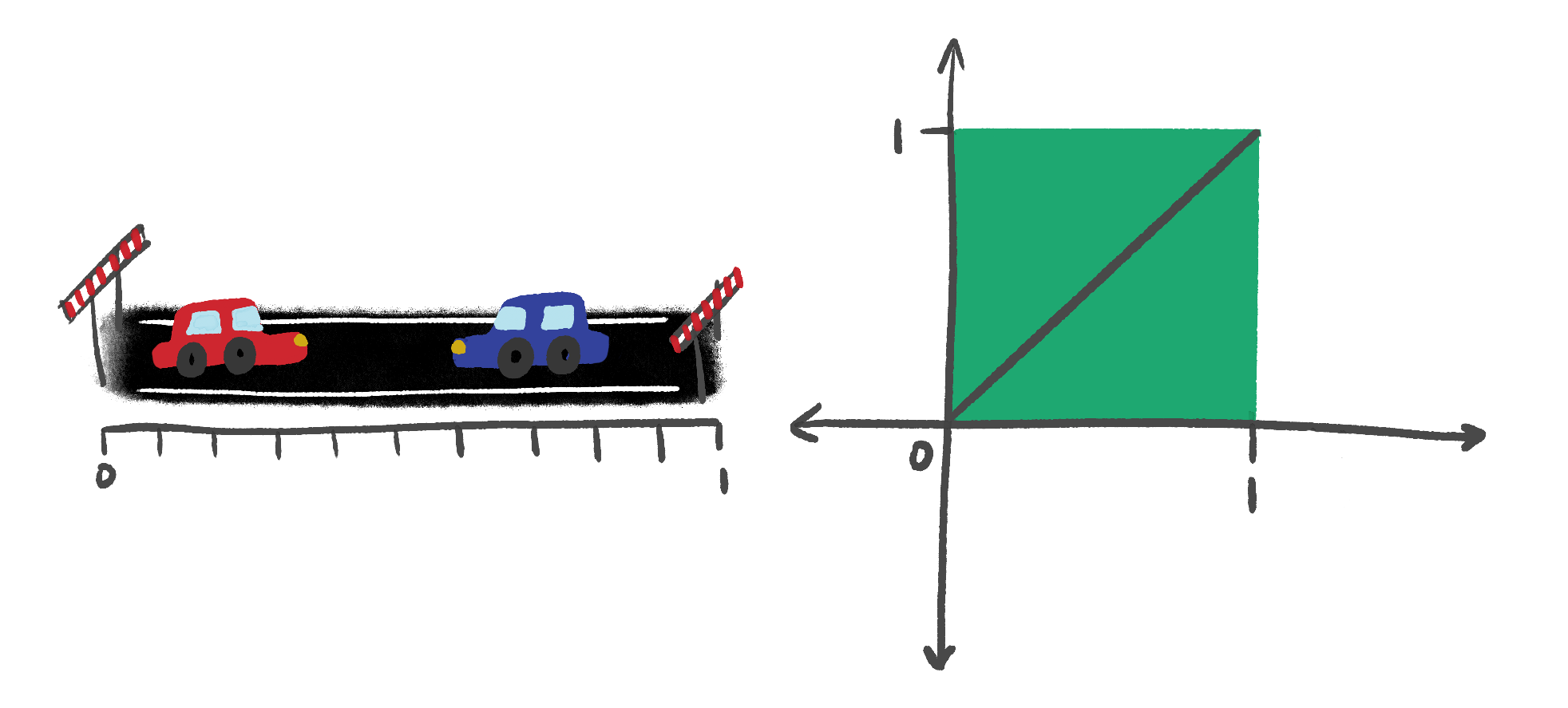
Imagine driving down a narrow road with cars parked on both sides. Suddenly you meet another car driving in the opposite direction. First, you look around for a space to pull over, but you have no luck. So you are forced to back up until you reach the next intersection so that you and the other car can pass each other. Thankfully cars can drive in reverse!
But now we construct a nightmarish hypothetical by placing two cars on a one-lane road with dead ends on both sides. The poor cars can never switch places by driving. We can see this by building another space to model the situation.
The configuration space is the set of all possible positions of the two cars on the road—including those reachable if we, acting like a child with toy cars, pick them up and place them down again. We can designate each car’s position by a number between 0 and 1: we give ‘0’ to the West end of the road and ‘1’ to the East end. Then each configuration is given by a point in \(\mathbb R^2\) of the form \[(\text{position of car A}, \text{ position of car B}).\] In total, the configuration space consists of all points in the unit square \([0,1] \times [0,1]\) except for the diagonal (points of the form \((x,x)\)) since the two cars must be in different positions. The fact that the two cars cannot switch their positions (by themselves) is shown by how the configuration space is not connected.
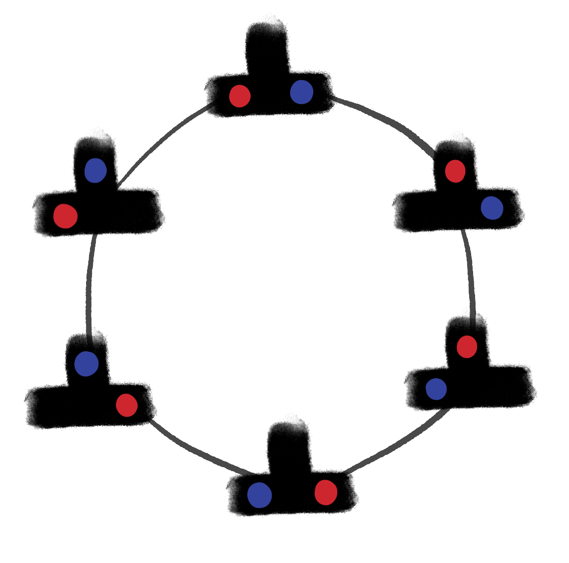
Now we mercifully add an alley partway down the road. Then one car can pull aside to let the other pass and thus, all configurations of the two cars on this road can be reached by driving. This means that its configuration space is connected. We can build a model of this configuration space by taking a few of the positions and connecting them by paths if they are definitely reachable by driving.
Whether a space is connected or not is a very coarse description; there are some more refined questions we can ask. Topologists are interested in getting information about a space by extracting some algebraic structure. One such object we will look at today is the fundamental group.
A brief description of the fundamental group
Suppose you are walking a dog on a leash in a field with a tree in the middle. Suddenly Fido bolts off to chase a squirrel, but you stand still in astonishment. Ten seconds later, you call him and he comes running back. Whether or not he made a lap around the tree will make a big difference for you! If not, you can easily pull the leash tight. But if he has, then now you have to go around the tree to untangle the leash. If the squirrel ran around the tree several times and Fido followed him, you will have to make several circles to untangle the leash. For you, the exact path that Fido made does not matter. You only care about the number of times (and in which direction) you now have to walk around the tree.
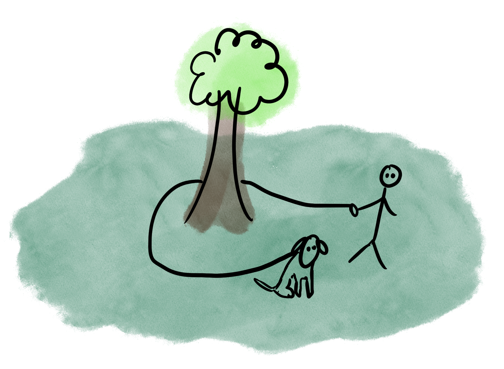
The fundamental group consists of loops up to wiggling and contracting, which mathematicians call homotopy. This wiggling and contracting is like pulling the leash tight after Fido’s joy-run. And from our little thought experiment, we see that each loop is characterized by the number of times and the direction it wraps around the tree (we can choose positive numbers for counterclockwise wraps and negative numbers for clockwise wraps). Also, loops add in the same way integers do. If Fido runs once around the tree, twice, it is the same as if he ran two times around the tree. (1 + 1 = 2) If he runs around once around clockwise and once around counterclockwise, he will untangle the leash himself. (1 + -1 = 0)
From this, we can see that the fundamental group of the field with the tree is the integers \(\mathbb Z\). And likewise, the fundamental group of the configuration space of the second road— the one with the alley— is also \(\mathbb Z\).
Dancers on stage
Let’s look at a more complicated configuration space. Imagine a group of \(k\) dancers on a stage. We will consider the configuration space consisting of all positions of those dancers. We will not be concerned with placement of each dancer’s limbs, but will instead only keep track of their spot on the 2-dimensional stage. Certainly the configuration space is connected since the dancers can get from any one configuration to any other. So let’s try to find the fundamental group to get more information.
To simplify this situation, we will model each of the \(k\) dancers as a point in \(\mathbb R^2\). Then the configuration space consists of all lists of \(k\) distinct points in the plane. It is written as \[\mathop{\mathrm{Conf}}_k(\mathbb R^2) := \{(a_1, \dots, a_k) \: | \: a_i \in \mathbb R^2, \: a_i \neq a_j \text{ if } i \neq j\}.\] A loop in \(\mathop{\mathrm{Conf}}_k(\mathbb R^2)\) corresponds to a movement sequence where every dancer returns to their starting position. How can we record such a dance? We could record a video of the dancers, but when we watch it, we will only see one frame at a time. Instead, we can introduce another dimension.
Suppose we have a video of the points moving in the plane which corresponds to the dance. It starts at time 0 and ends at time 1. Then we slice it into many frames and lay them on top of each other with the first frame on the top of the stack and the last frame at the bottom.
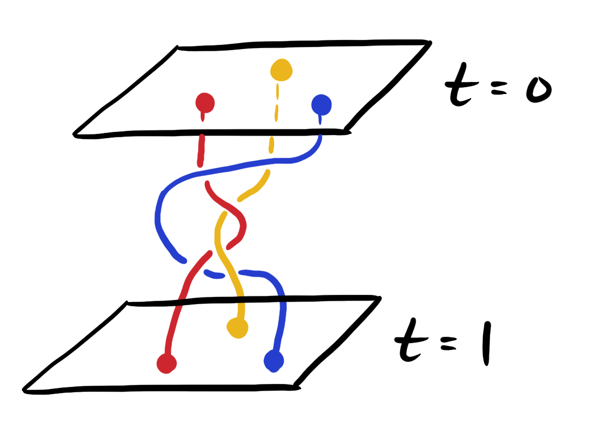
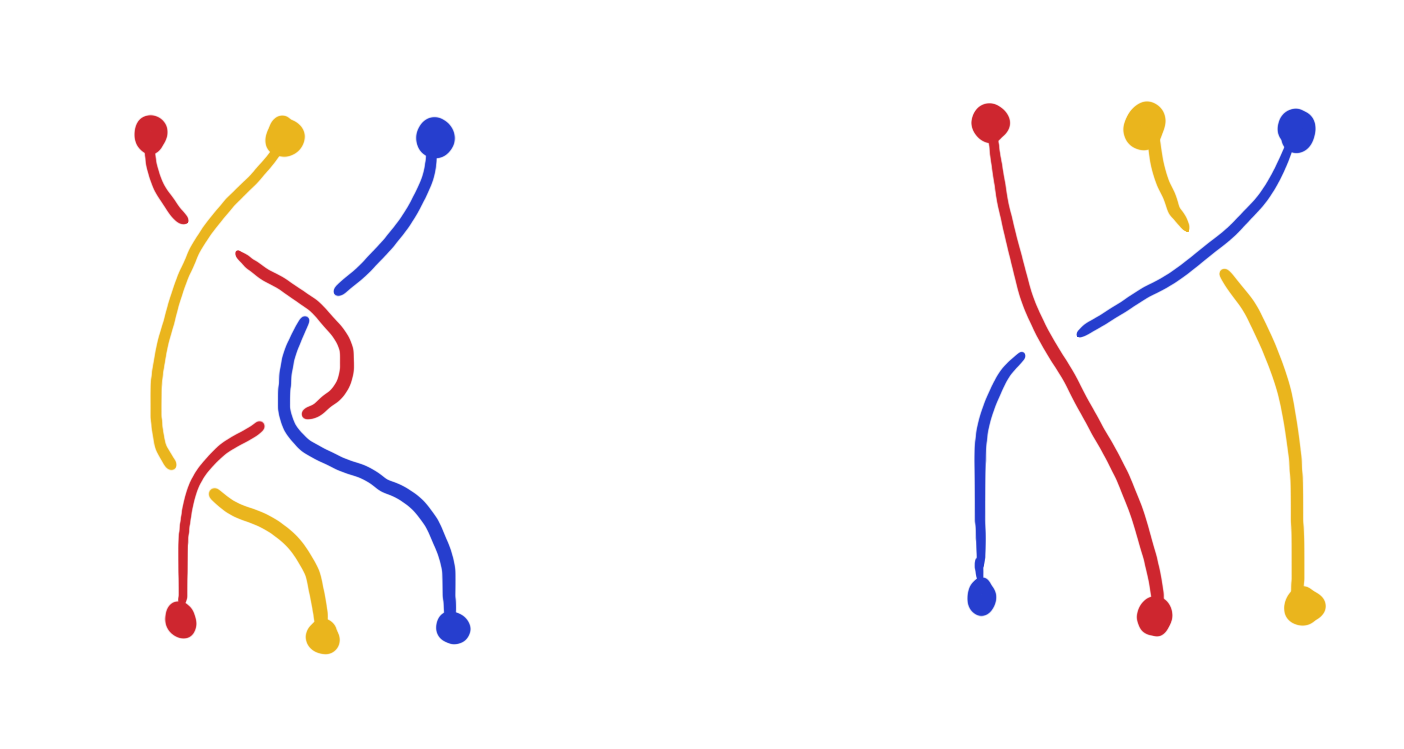
If we track one point moving from \(t = 0\) to \(t = 1\), it will trace out a curve in space. The curves will weave around each other like braiding strings. In this way, each loop in the configuration space can be realized as a braid on \(k\) strands.
The braid group
A braid is a weaving of \(k\) strands in three-dimensional space with the top ends pinned in a starting position. There are some braids where the strands return to their starting order at the end of the braid; we call these perfect braids.
For a point \((a_1, \dots a_k)\) in our configuration space, either we care about the order of these \(k\) entries, or we don’t. In our dance metaphor, this is the difference between dancers who are each in a unique costume and distinguishable vs. dancers who are in uniform costume and indistinguishable.
Mathematically speaking, what we have already defined is the ordered configuration space. The unordered configuration space \(\mathop{\mathrm{UConf}}_k(\mathbb R^2)\) is given by \(\mathop{\mathrm{Conf}}_k(\mathbb R^2) / S_n\) where \(S_n\) is the symmetric group and it acts by permuting the points. Loops in \(\mathop{\mathrm{Conf}}_k(\mathbb R^2)\) correspond with perfect braids, where all strands come back to their own spot. And loops in \(\mathop{\mathrm{UConf}}_k(\mathbb R^2)\) correspond with braids where strands return to any spot.
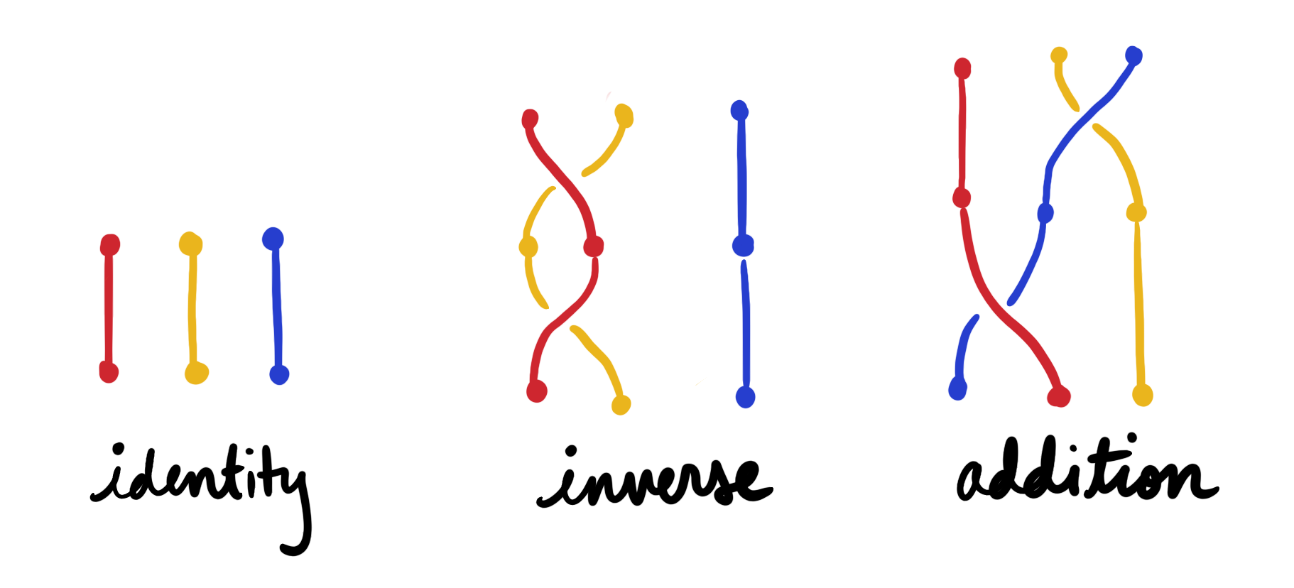
Then we note that braids do form a group. The identity is given by keeping all strands straight. The inverse of a braid is given by reflecting the braid across the vertical axis. Two braids are added by stacking one on top of another. I will leave you to think about why the collection of pure braids forms a subgroup of all braids.
So we have explained (but not showed) that the fundamental group of \(\mathop{\mathrm{UConf}}_k(\mathbb R^2)\) is the braid group on \(k\) strands, denoted \(B_k\). And the fundamental group of \(\mathop{\mathrm{Conf}}_k(\mathbb R^2)\) is the pure braid group on \(k\) strands, denoted \(P_k\).
I love this piece of math because \(\mathop{\mathrm{Conf}}_k(\mathbb R^2)\) seems like a highly inaccessible space. It contains \(2k\) dimensions since there are 2 coordinates specified for the location of each of the \(k\) points. However, by changing perspective, we find that its fundamental group is a very understandable and beautiful object. This is one example of how topology can help us access the inaccessible.
 Fran Herr is a PhD student in mathematics at the University of Chicago. She studies low dimensional topology and geometric group theory. You can follow her on YouTube and X.
Matt Enlow – A Sine Surprise
Note: I drafted all four of my pitches before the Big Math-Off started, because I knew that I would not have time to write them “on demand.” What I did not count on was the possibility that another participant would choose one of my four “cool math things” to talk about in one of their pitches. Yet this is what has happened! What are the odds?!? (No, seriously.) I decided to just forge ahead as planned, present my pitch, and let the voters decide how much the déjà vu matters to them. Thank you for understanding, and enjoy!
I remember the moment that my antipathy towards calculators began. I had only been teaching for a year or two (we won’t talk about which century this was), and I was teaching a summer school class. When I saw a student—a sophomore in high school—reach for his calculator to determine the value of \(6 \times 7\), I may have involuntarily let out a small shriek.
In retrospect, that may not have been the most empathetic response. But ever since then I have had to work hard to overcome my fuddy-duddy-Luddy bitterness over what the ubiquity of calculators has done to the learning—and, yes, the enjoyment—of mathematics.
But in today’s excursion, I admit an exception to that bitterness, and present to you a phenomenon that quite possibly would have never occurred to the Eulers or Archimedeses of history, due to the severe lack of digital calculators at the time.
Let’s Begin!
Please take a moment to try to locate for yourself a scientific calculator. It must satisfy the following requirements:
It must have buttons for trigonometric functions (“sin,” “cos,” and “tan”).
It must be in “Degree Mode,” meaning that it will interpret any argument fed to a trig function as being an angle measured in degrees (rather than radians). If entering
sin(90)gives you1, rather than0.893997, then you’re all set!It must automatically write sufficiently large or small numerical results using scientific notation (such as
6.022x10²³or6.022e23).
(If you don’t have such a calculator handy, don’t worry. I got you.)
Now I would like you to evaluate, in turn, each of the following expressions, noting the outputs:

Take your time. I’ll be right here.
For those without calculators, the animation below is a fairly good simulation of what you might have experienced:
*Ahem* Allow me:
WHAT.
ON.
EARTH…
… is \(\pi\) doing here?!? WHY?!? WHAT?!? HOW?!? What the heck do numbers that are just strings of 5’s have to do with \(\pi\)?!?
Before we proceed, let’s just take a moment. This shock, this bafflement, this magic, this wonder, this mystery—this is what keeps mathematicians doing mathematics. Yes, we’ll eventually look into it a little more closely, and get some of our “Why” questions answered, but this moment, this not-knowing, this state of being mystified, this reminder that the universe still holds so much magic in it, is worth savoring.
And no matter how many times you have this experience, mathematics will always have more in store.
Stating Our Claim
Okay, so what is going on here? Let’s start by trying to state what it is that we’re seeing:
As the number of 5’s in the denominator increases,
\(\sin\!\left(\frac{1}{555\ldots 5}^{\circ}\right)\) approaches \(\pi\) times 10 to some negative power.
This is okay for a first pass, but we can do better. For example: Is there a relationship between the number of fives we use and the exponent on 10 in the result? An examination of our data seems to suggest that if we use \(n\) 5’s, then the exponent on 10 will be \(-(n+2)\).
Now… Can we write an expression, in terms of \(n\), for a number written as a string of \(n\) 5’s? We can, by making use of the fact that the number \(\underbrace{999 \ldots 9}_{n\text{ 9’s}}\) can be written as \(10^n-1\). This means that
\[\underbrace{555 \ldots 5}_{n\text{ 5’s}} = \frac{5}{9}(10^n-1),\]
and its reciprocal, \(\frac{1}{555 \ldots 5}\), can be written as \(\frac{9}{5(10^n-1)}.\)
So now we can rewrite our claim more precisely:
As \(n \rightarrow \infty\), \(\sin\!\left(\frac{9}{5(10^n-1)}^{\circ}\right) \rightarrow \pi \times 10^{-(n+2)}\).
Next comes the piece that really makes the trick “work.”
Radians vs. Degrees
One fact about the sine function is that when you give it an input value close to zero, the output is very close to the input. Stated more precisely:
As \(x \rightarrow 0\), \(\sin(x) \rightarrow x\).
However, this statement is only true if \(x\) is measured in radians.
In each of the graphs below, the graphs of \(y=x\) and \(y=\sin x\) are plotted.

Note that when \(x\) is in radians, the two graphs almost coincide near \(x=0\), but when \(x\) is in degrees, the two graphs are very different.
It’s clear that the successive inputs that we fed our calculator were approaching zero. But we need to look at what those inputs of \(\frac{1}{555…5}\) degrees look like when they are converted to radians. We can do this using the conversion factor \(\frac{\pi\text{ radians}}{180^{\circ}}\):
\[\left(\frac{9}{5(10^n-1)}\right)^{\circ} =\left(\frac{9}{5(10^n-1)}\right)^{\circ}\times\frac{\pi\text{ radians}}{180^{\circ}} =\frac{\pi}{100(10^n-1)}\text{ radians}\]
Aha! (… This is the part where you yell “AHA!” really loudly.) Suddenly all of our fives and nines have disappeared, and it’s powers of 10 as far as the eye can see.
As \(n\) approaches infinity, we can see that this latter expression approaches \(\frac{\pi}{100(10^n)}\), or \(\pi \times 10^{-(n+2)}.\) And with this, we have proven our claim that
As \(n \rightarrow \infty\), \(\sin\!\left(\frac{1}{555…5}^{\circ}\right) \rightarrow \pi \times 10^{-(n+2)}\).
So, looking back… What made this “trick” so surprising? It really just seems to come down to the human-introduced division of a circle into 360 pieces. So one thing this might lead one to wonder is whether similar tricks would exist if we had decided to use a unit of angle measurement that divided a circle into a different number of parts. For example, a less-frequently-used unit of angle measurement (in mathematics, anyway) is the gradian. There are 400 gradians in a full circle. Could you create a similar trick with a calculator that’s in “gradian mode?” If not, what subdivisions of circles would easily lend themselves to such a trick?
As always, there are plenty of other directions our wondering brains might go, and I hope you chase those rabbits to your hearts’ content and delight.
 Matt Enlow teaches mathematics at the Dana Hall School in Wellesley, MA. You can follow him on X, BlueSky and Mathstodon.
So, which bit of maths has tickled your fancy the most? Vote now!
Semi-final 1: Fran Herr vs Matt Enlow
- A sine surprise (and a sense of déjà-vu)
- (69%, 146 Votes)
- Configuration spaces
- (31%, 67 Votes)
Total Voters: 213
This poll is closed.
The poll closes at 08:00 BST tomorrow. Whoever wins the most votes will get the chance to tell us about more fun maths in the final!
Come back tomorrow for the other semi-final match, pitting Angela Tabiri against Ayliean, or check out the announcement post for your follow-along wall chart!