This is the eleventh match in our group stage: from Group 1, it’s Jim Propp up against Sophie Carr. The pitches are below, and at the end of this post there’s a poll where you can vote for your favourite bit of maths.

Take a look at both pitches, vote for the bit of maths that made you do the loudest “Aha!”, and if you know any more cool facts about either of the topics presented here, please write a comment below!

Jim Propp – The Sphere Packing Problem

Jim Propp is a math researcher/teacher/popularizer on the faculty of the University of Massachusetts Lowell who blogs at Mathematical Enchantments. Jim is active in the Gathering 4 Gardner Foundation, the Global Math Project, and the National Museum of Mathematics. He’s @JimPropp on Twitter.

Is there a way to pack more than 4 disks of diameter 1 into a 2-by-2 square?

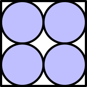
Obviously not. But is there a way to pack more than 4000 disks of diameter 1 into a 2-by-2000 rectangle?

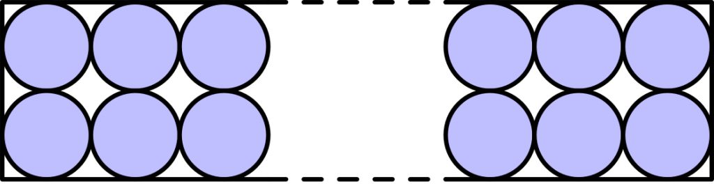
Again, obviously not — except that there is a way! (See my essay “Believe It, Then Don’t” for details.) So packing problems can be tricky.

If you’re packing equal-size disks into a large region, it’s intuitive that the best way to pack them is six-around-one. This is the hexagonal packing, and László Fejes Tóth showed in 1940 that it’s the best way to pack the infinite plane. Here the word “best” needs to be unpacked (pardon the pun), since both the hexagonal packing and the square packing fit infinitely many disks into the plane.

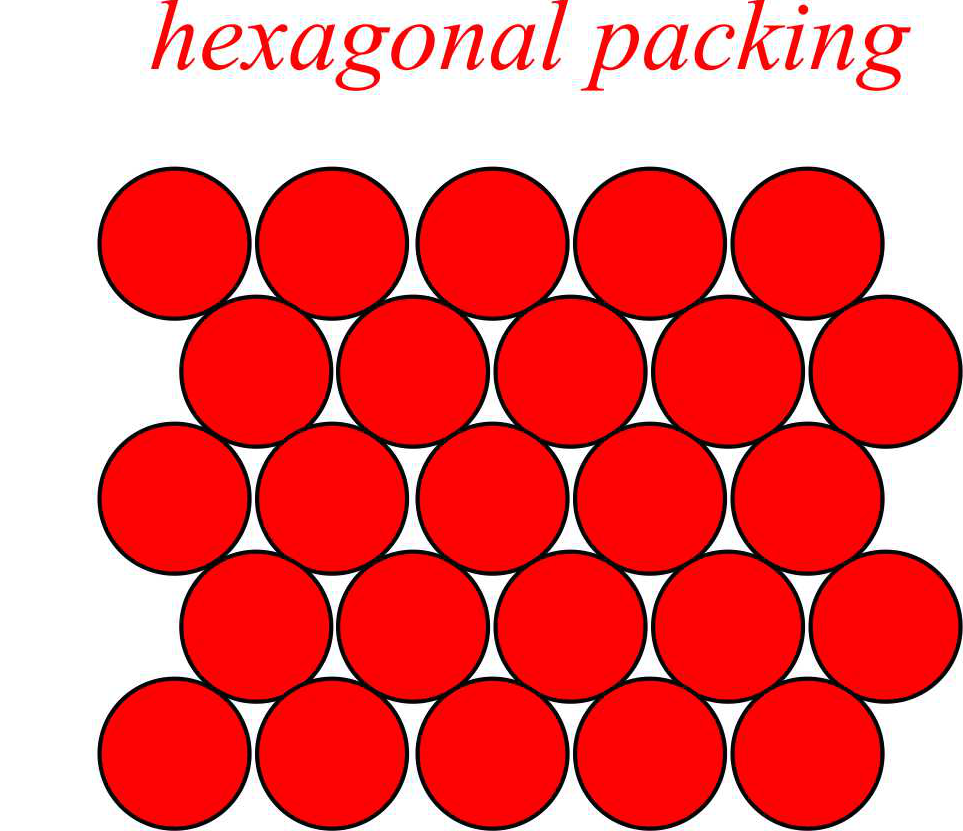
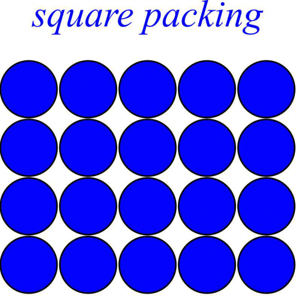
The way in which the hexagonal packing beats the square packing is that the former fills about 91% of the plane (more precisely $\pi \frac{\sqrt{3}}{6}$) while the latter fills only about 79% of the plane (more precisely $\pi/4$). That is, the hexagonal packing has a larger packing fraction. To compute the packing fraction of the square packing, divide the plane into $2r$-by-$2r$ squares where $r$ is the radius of the disks.

Each square has area $(2r)^2 = 4r^2$ and contains a disk of area $\pi r^2$, so the packing fraction in each square is $(\pi r^2) / (4r^2) = \pi/4$ (notice that the radius drops out of the formula). Likewise you can compute the packing fraction of the hexagonal packing by dividing the plane into hexagons.

What about packing spheres in three-dimensional space?

Let’s write points as triples of numbers. If we take all the points $(a,b,c)$ for which $a$, $b$, and $c$ are integers, no two of the points are closer than distance 1, so we can put spheres of radius 1/2 around each of them and the spheres don’t overlap. (If two points are at distance $d$ from one another, spheres of radius $d/2$ centered at the two points will touch but won’t overlap.) The sphere centered at $(a,b,c)$ is tangent to the spheres centered at the six points $(a \pm1, b, c)$, $(a, b \pm 1, c)$, $(a,b,c \pm 1)$. This gives us the cubical packing, and it covers about 52% (more precisely $\pi/6$) of 3-dimensional space.

Not bad! But it turns out that if you throw out half of the spheres and inflate the rest, you can get a bigger packing fraction. Here’s how it works. Imagine painting those spheres red and blue, where a sphere centered at $(a,b,c)$ is red if $a+b+c$ is even and blue if $a+b+c$ is odd. Each red sphere touches six blue spheres. If we cull the blue spheres, then no red sphere touches any other sphere, so there’s room for us to expand the radii of the red spheres. By how much? The nearest neighbors of the red sphere centered at $(a,b,c)$ are now the twelve red spheres centered at $(a \pm 1, b \pm 1, c)$, $(a \pm 1, b, c \pm 1)$, and $(a, b \pm 1, c \pm 1)$; these twelve points are all at distance $\sqrt{2}$ from the point $(a,b,c)$, so we can expand the radii of the red spheres from 1 to $\frac{\sqrt{2}}{2}$ and the red spheres still won’t overlap (though they will graze each other). This is a win because the volume of a sphere grows like the cube of radius. That is, even though the packing fraction went down by a factor of 2 when we culled the blue spheres, it went up by a factor of $(\sqrt{2})^3 = 2 \sqrt{2} \gt 2$ when we inflated the red spheres. So our new culled-and-inflated packing has a bigger packing fraction (bigger by a factor of $\sqrt{2}$), namely $\pi \frac{\sqrt{2)}}{6}$, or about 74%.

Is this packing the best possible? Johannes Kepler thought it was, and for centuries, nobody could find a better packing but nobody could prove that there wasn’t one. It wasn’t until 2005 that Thomas Hales published a proof that Kepler’s packing fraction can’t be improved.

What about packing spheres in four-dimensional space? What would that even mean? If we relinquish visualization and rely on analogy, we can just define four-dimensional space as the set of quadruples $(a,b,c,d)$ of real numbers, and define the distance between two quadruples $(a,b,c,d)$ and $(a’,b’,c’,d’)$ as

\[ \sqrt{(a-a’)^2 + (b-b’)^2 + (c-c’)^2 + (d-d’)^2} \]

and so on. Then we can use the same trick that worked in three dimensions. Take a hypersphere centered at each point $(a,b,c,d)$ where $a$, $b$, $c$, $d$ are integers, and paint it red or blue according to whether $a+b+c+d$ is even or odd. If we cull the blue hyperspheres and inflate the red hyperspheres by a factor of $\sqrt{2}$, we get a packing that’s exactly twice as dense as the 4-dimensional hypercubical packing. This is called the $D_4$ packing, and it’s believed to be optimal, but nobody has proved it.

You might think you can guess how the rest of the story goes: 5-dimensional packing is even harder than 4-dimensional packing, 6-dimensional packing is harder still, and so on, forever. But no! That’s the thing I find most amazing about this story. For two special values of $n$, mathematicians have been able to prove that the densest known way to pack $n$-dimensional hyperspheres is in fact the densest possible way. These exceptional dimensions are $n=8$ and $n=24$. The proof for $n=8$ was found by in 2016 by Maryna Viazovska, and the proof for $n=24$ was found a week later by Viazovska in collaboration with Henry Cohn, Abhinav Kumar, Stephen Miller, and Danylo Radchenko. Erica Klarreich’s article is a great place to look if you want to know more. Or check out Kelsey Houston-Edwards’ Infinite Series video about sphere-packing.

One thing I love about this topic is that despite the sophistication of the methods used by Viazovska and her collaborators, the subject is still in its infancy. The only dimensions we understand right now are 1, 2, 3, 8, and 24. I’m guessing that the 4-dimensional case is the one somebody will solve next, but who knows?

Sophie Carr – Navier-Stokes

Sophie Carr is the founder of Bays Consulting. Having grown up building Lego spaceships she studied aeronautical engineering before discovering Bayesian Belief Networks which has led to a career she loves – essentially make a living out of finding patterns. She prefers fresh coffee over tea, pears over apples and her favourite flower is the tulip. She’s @SophieBays on Twitter.

Bernoulli’s equation really sparked an interest in maths (albeit learnt in an A Level Physics lesson) and at 18 I went off to study Aeronautical Engineering and then Applied Maths and Fluid Mechanics. It’s this part of my life that the second equation that always makes me smile appeared and what I’m going to talk about in this post.

I honestly worked really hard at my studies but when I need to switch off, I’ve long turned to a good puzzle. There is something absorbing about puzzle solving and literally only once have I solved The Times cryptic crossword – to achieve this I was part of a team and we didn’t win the prize that week (the team was formed during a less than favourite subject tutorial and it took us a whole year to learn the patterns of the crossword writers so we could complete the crossword in the hour available to us) I do manage maths puzzles on my own, but I’ve never won any money for them – the result has been a slightly happier bounce in my step as I go to put the kettle on. However, if you look around you can win a substantial amount of money for solving a maths puzzle. In fact, you could win $1,000,000 (but more importantly you’d get that really great feeling when you actually solve a puzzle).

At the start of this century, The Clay Mathematics Institute announced a series of problems called “The Millennium Problems” and these were the seven trickiest problems in maths at the time. All the problems had been studied for a long time, in fact the Reimann Hypothesis was already being talked about as a tricky problem in 1900. Although really challenging, the problems aren’t impossible: one, The Point Carre Conjecture, has been solved.

Now I will openly admit that I don’t understand many of The Millennium Problems and I’m certainly not about to solve any of them myself. That said, there is a problem you don’t actually have to solve to get the prize- you just have to make “substantial progress toward a mathematical theory which will unlock the secrets hidden….”. What problem could possibly be so tricky yet alluring? The answer is one of the key equations in fluid mechanics – the Navier-Stokes Equation .

Simply put the Navier-Stokes equation models any moving fluid – whether they be liquids or gases: from glaciers to the air we breathe. At the heart of the equation is an extension of Newton’s second law of motion:

\[ \text{Mass} \times \text{Acceleration} = \text{Force} \]

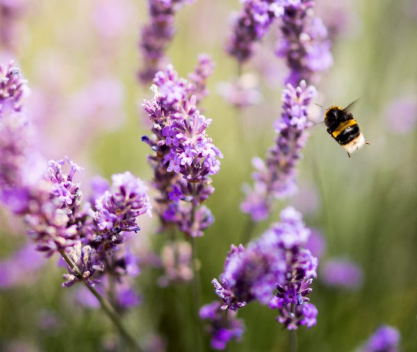
I think of the Navier-Stokes equation as a bumble-bee. The theory says that the bumble bee can’t fly, yet it does. The Navier-Stokes equation does a brilliant job at explaining and predicting what we see when fluids flow, but it can’t explain how the fluid actually moves. Therein lies the tricky problem that still needs to be solved. So who’s up for a challenge?

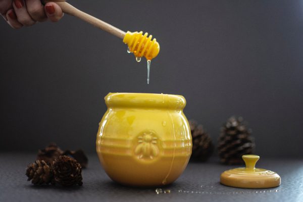
A good place to start is how the equation was developed, which was by Euler representing the flow of a steady (no turbulence or swirling) incompressible (the density of the fluid doesn’t alter with pressure) fluid. From this starting point, an engineer, Claude-Louis Navier, developed Euler’s initial equation to include viscosity. This was (and still is) really important because often when people think of a fluid flow, they think of water moving. But what about fluids like honey, ketchup, mayonnaise or hair gel? They are much thicker (viscous) than water and move in different ways – in fact some fluids, called Non-Newtonian fluids, even change how they move when stress or strain is applied (a great example of this is Oobleck and if you’ve never made it, I can heartily recommend it as a messy way to spend an afternoon) In modern life we use viscous an Non-Newtonian fluids all the time. Moving these fluids through pipes and tubes is a really important engineering problem within production manufacturing.

About 20 years after Claude-Louis, Sir George Gabriel Stokes, a British physicist and mathematician, further developed the fluid flow equation and produced a complete (also known as a general) solution for two dimensional flow. Only we don’t live in a two dimensional world, and that is where the problems arise.

To be accurate at this point I need to stop talking about the Navier-Stokes equation and start talking about the Navier-Stokes equations because we need to think about the fluid moving in all three directions: up/down; left/right and back/forth. Often it’s easiest to think of a small volume of a fluid, which is frequently drawn as a cube. Personally, I always think of this little cube of fluid like a cube of sponge. This helps me visualise what will happen to the volume of fluid when an external force or a viscous stress is applied from any direction, for example the cube could change shape or velocity. Now I’m not sure if this is the best way to think of the fluid, but it’s helped me understand how each little bit of the fluid can be affected and move. If you’ve got any tips on this, please share!

So how can we take Newton’s second law and extend this into something which models viscous fluid flow in three dimensions?

\[ \text{Mass} \times \text{Acceleration} = \text{Force} \]

Well from the above equation, the Navier-Stokes equations can be summarised as:

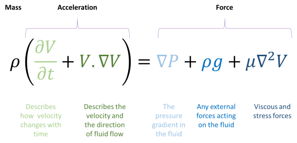
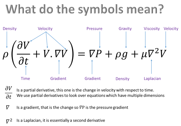
This one equation is actually a series of equations which captures the fluid moving in three dimensions through the use of partial derivatives and something called the Laplacian. The mass of the fluid is represented by its density and acceleration is the change of velocity with time. The overall force is the total of pressure gradient, stress caused by the viscosity/fluid particles bumping into each one another and any other external forces.

So far, so good. The problem starts when we think about the acceleration of a fluid. As in life, fluids can move along steadily and calmly. No upsets, swirling or turbulence. In fact a nice laminar flow is akin to a team all working together in unison. All the parts of the fluid (or team) moves in the same direction and there’s an even distribution of work.

However, quite literally, life isn’t always plain sailing and something causes an upset – in our analogy the team stop all working well together and in the fluid we’re thinking about, flow stops being smooth. Within the fluid, work stops being evenly distributed: small pockets of the flow literally starts to move in different directions and within the pockets energy becomes really concentrated and the flow starts to swirl. This is called and eddy and the forming eddies break off from the main body of the moving fluid. Within the formed eddies more and more eddies form, creating more turbulence and chaotic looking flow.

What’s amazing is that overall (and all things being considered) the Navier-Stokes equations do a really great job in predicting what the flow is going to look like, even in three dimensions of the real world. So what’s the problem with calculating the acceleration?

As we consider the eddies and the fluid flow on a smaller and smaller scale, the velocity of the volume of fluid were thinking about becomes faster and faster. Eventually a point is reached where the velocity of the fluid is, in theory, infinite. The impact of that is that you can no longer calculate an acceleration, because acceleration is the rate of change of velocity with time. You can’t calculate the rate of change of an infinite velocity. At this point you can no longer use the equation – in fact the rather impressive term is that the equation “blows up”.

So we now have a conundrum. An equation that is like a bumble bee. Nature shows the bumble bee flying and fluids happily moving along. We have an equation that can predict what a fluid flow will look like in the real world, but can only be genuinely solved in two dimensions – not the messy world we actually live in. Instead we rely on numerical analysis methods (these are a wide range of methods which looked for a converged solution to a problem that can’t be “exactly” solved) because we get to a point in turbulent flow where the equation blows up.

This is, to me at least, just so cool. We use the results of an equation which we can’t actually prove is correct, that has to be approximated using complex numerical methods on some of the most complex applied maths and engineering problems we face. The Navier-Stokes equations are used to design engines, aeroplanes and ships. The video below shows a lifting aerofoil (and thanks to The IMA for the use of the demonstration) and calculating the lift force is achieved through the use of the Navier-Stokes equations.

The equations are used to model the flow of all sorts of fluids through pipers, the flow in rivers and streams and crucial to everyone, to model weather patterns. Quite literally, making substantial progress on the Navier-Stokes equation will impact every single person’s lives. That has to be worth the effort. Tricky, yes. But just think of how satisfying it will feel to actually solve them – just how high would the bounce in your step be as you walked to pop the kettle on?

So, which bit of maths do you want to win? Vote now!

 Loading ...

The poll closes at 9am BST on the 12th. Whoever wins the most votes will win the match, and once the group stages are over, the number of wins will determine who goes through to the semi-final.

Come back tomorrow for our twelfth match of the group stages, featuring Kyle Evans and Becky Warren. Or check out the announcement post for your follow-along wall chart!