Here we are! It’s finally the final! One month and 52 pieces of fun maths later, we’re just two more bits of maths away from finding the identity of The World’s Most Interesting Mathematician (2019, of the 16 people I asked to take part, who said yes and were free in July).
It’s Sameer Shah facing up against Sophie Carr. This match works like all the others: they’ve each got a pitch about something mathematical that interests them, and your job is to vote for the the one that makes you go ‘aha!’ the loudest.
Sameer Shah – Round 5

Sameer Shah has been teaching high school math in Brooklyn for the past twelve years. You can read his musings about his classroom at Continuous Everywhere but Differentiable Nowhere. He’s @samjshah2 on Twitter.
The Big Internet Math Off 2019 is coming to a fast close and honestly, I didn’t think I would get here or close to here. I just want to take a moment to sincerely gush over all the posts and writers. The first thing I do each day when waking up is go read two mathematical gems. A lot were new to me and some I had seen — but it is how people chose to make their favorite mathematical things accessible, interesting, in their own voice that I love most. Anyone who thinks math might be this sterile thing merely has to see these entries through my eyes, and experience my brain exploding, to know that math is anything but. (And as @honeypisquared suggested in her semifinal pitch, we want MOAR and MOAR people to have those experiences, where the umbrella of what gets counted as math gets wider and more inclusive.) So from this humble high school teacher, thank you everyone who shared a bit of something they are passionate about, that they care about, with us. In some weird metaphorical way, it’s like you were giving us a bit of you, and I am grateful. Okay, weird, awkward, overly impassioned moment over.
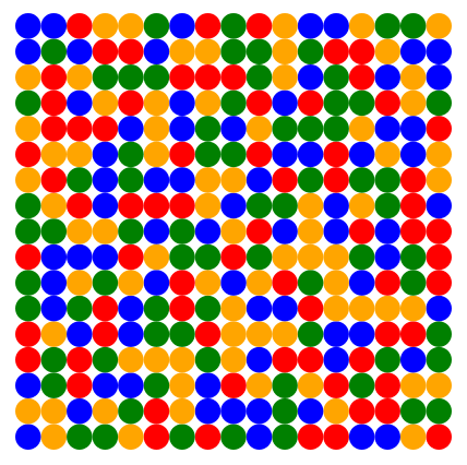
I have only one last chance to share with you something interesting. My last bit of maths is going to be to show you two squares. The first is a
Both are beautiful to me in different ways. With somewhat joking confidence, I can officially say that these two squares are the most beautiful
As someone who enjoys modern art and vibrant colors (for example, I love Josef Albers’ Homage to the Square series), the
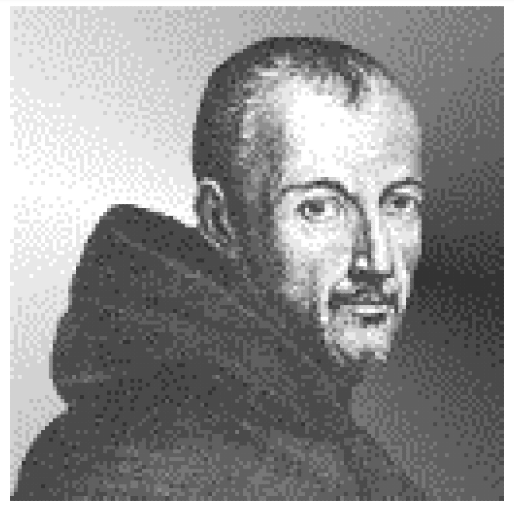
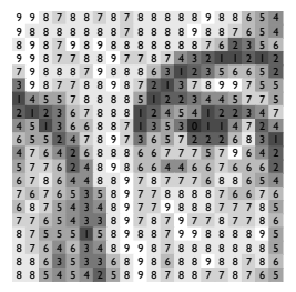
Initially, I don’t love the second square. I’m first struck by how pixelated it is, how low-res it is, like it was displayed on a 1990s Geocities website, chosen for easy loading. It feels old in that sense, and also ancient in the subject being portrayed. It’s not my style square, ya know? At least not initially. Oh, the subject is an image of Marin Mersenne — who a class of prime numbers are named after — but also was a priest, music theorist, and central node in a network of seventeenth century mathematicians and scientists. The longer I look, though, the less I see the subject and the more I think how about neat it is that we can capture an image, a painting, so efficiently with only
But yeah, that’s not all these squares have to offer. They each have deeply embedded mathematics in them. Ready to have your mind blown?
Look at the colorful square. There’s something wonderfully unique about it, and took years for someone to discover it. It seems like the coloring is random, but it isn’t. If you haven’t yet had a chance to stare at it for 90 seconds and “notice” and “wonder,” take some time to do so. See if you can’t find something interesting about it. I’ll seriously wait for you to do that!
Waiting… waiting…
Now I’m going to change just one of the colors:
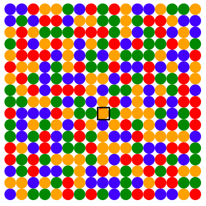
The new version of the square is broken. The image is RUINED for me. It doesn’t have the mathematical property that makes the first grid the most beautiful
Look at
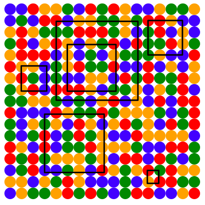
But maybe your obsession with squares wanes a little, and you start looking at
Okay, okay, you can’t do a rectangle that is a 1xn rectangle. That’s like a line segment. I’m talking a true rectangle.
You’ll find in the original square, you can’t ever draw a rectangle with four corners having the same color. But in my slightly sullied square, you can. (In fact, I found two rectangles each with four yellow corners in that abomination!)
The original square has hidden depths, y’all. I first saw this on Brett Yorgey’s blog The Math Less Traveled around 2012-ish (I took the image I’ve shared with you from that page) and posted the
There’s also this game that exists that has you “fix” squares by changing their colors until all rectangles disappear.
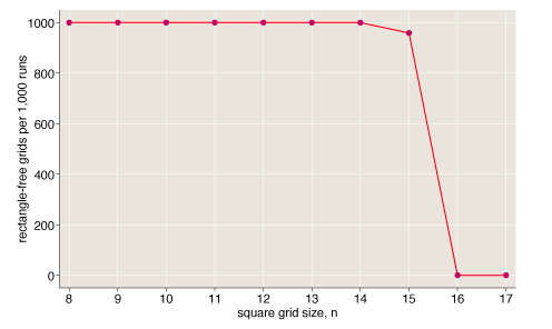
He generated 1,000 random colorings (using four colors) of
It turns out that since then, researchers have figured out things more generally: if you have 4 colors and an
Think of your first glance at that vibrant
Now the
So yeah, it turns out that if we look at the 16,129-digit number created by the image, it turns out that this number is a prime number. Remember our dear Mersenne is known now for a class of prime numbers!!! Think about that while looking at the image again!
It just so happens that THERE IS A PRIME NUMBER THAT WHEN ITS DIGITS ARE TURNED TO GREYSCALE HAPPEN TO FORM THIS IMAGE OF MERSENNE, WHO IS KNOWN TODAY FOR PRIME NUMBERS.
When I first saw this, I felt a sense of wonderment and bafflement… baffderment.
If you want to know how this beautiful
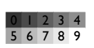
I found this image and the mathematics behind it in a four-page paper written by Zachary Abel for the 2016 Bridges Conference (a math-art conference). He exploited two basic premises: “primes are everywhere” and “primes are easy to spot (with a computer).” Starting with an image of Mersenne, he used a particular algorithm to convert it into a
How did Zachary know he was going to stumble into a prime number using this process? We know prime numbers are frequent for small numbers (e.g. 2, 3, 5, 7) but much more spread apart as we get to higher numbers (e.g. 151, 157, 163, 173, 197). So it could be the case that when we get to numbers that 16,129 digits long, it would be almost impossible to find one because the prime numbers are so spread apart.
It turns out he only had to do this “add slight noise-convert to
That’s because of something called the Prime Number Theorem. It says that the number of primes less than a number
| Number of primes less than | Our estimate of number of primes less than | |
| 1000 | 168 | 145 |
| 10000 | 1229 | 1086 |
| 100000 | 9592 | 8686 |
| 1000000 | 78498 | 72382 |
| 10000000 | 664579 | 620420 |
| 100000000 | 5761455 | 5428681 |
So let’s get concrete about this. Let’s look at the number 1,000. The probability that a random integer between 1 and 1,000 is prime can be estimated as approximately
which in mathematical formulation is
Back to our problem. We have a
Just to be clear,
Where does this all lead us? Let’s not lose the forest for the trees! We were trying to figure out if by slightly changing the pixel values on the original image of Mersenne and then coming up with
And that’s how we ended up with an image of Mersenne that is numerically represented by a prime number. We come up with a 16,129 digit number to represent Mersenne, and then change that number slightly a bunch of times and check for primality. If you check enough altered numbers, because of the Prime Number Theorem, one of those altered numbers will almost definitely be prime.
Like before, I ask you to think of your first reaction that low-res
To me, these two square images are what a lot of math is about for me. There’s something I see initially one way, but the more I learn about and explore it, I can appreciate it more and gain access to hidden depths. And usually, if I’ve done something right, I can’t look at a math problem or concept and see the same thing I initially saw. I see more… I see multitudes. Maybe you too?
Sophie Carr – Testing for pregnancy

Sophie Carr is the founder of Bays Consulting. Having grown up building Lego spaceships she studied aeronautical engineering before discovering Bayesian Belief Networks which has led to a career she loves – essentially make a living out of finding patterns. She prefers fresh coffee over tea, pears over apples and her favourite flower is the tulip. She’s @SophieBays on Twitter.
Oh my word, I’m writing a pitch for the final of the “Big Internet Math Off” how to choose one last topic to talk about? I’ve decided to go back to basics starting with probability trees and ask a question that’s slightly different to one which is often posed:
Many pregnancy tests state that they are 99% accurate, that is of women who are actually pregnant the test will correctly identify the pregnancy in 99% of them. This means there is 1% of women who are pregnant that the test won’t correctly identify. Overall let’s suppose that 5% of women are pregnant. What is the probability that a woman chosen at random has a negative pregnancy test and is in fact pregnant? What we want to calculate is
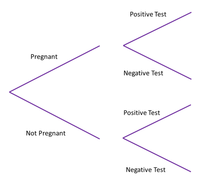
What this diagram succinctly shows is the impact of a test being just that, a test. It’s looking for evidence of being pregnant (increased hormone levels) and we need to separate that from actually being pregnant. On top of that, tests aren’t perfect, they occasionally pick up pregnancies that aren’t there (called a false positive) and miss pregnancies that are there (called a false negative). The differences in this context are summarised as:
| Hypothesis | ||
|---|---|---|
| Evidence | Pregnant | Not Pregnant |
| Pregnancy test is positive | True positive – pregnant and a positive pregnancy test | False positive – not pregnant but has a positive pregnancy test |
| Pregnancy test is negative | False negative – pregnant and a negative pregnancy test | True negative – not pregnant and a negative pregnancy test |
Each one of these: true positives, false positives, false negative and true negatives can be seen on the diagram. Even more, with the estimates we have for the accuracy of the test and the percentage of women who are pregnant, it is easier to understand how many women who have a negative pregnancy test but are pregnant if instead of probabilities we use frequencies. If we think of 10,000 women then if 5% of these are pregnant a total of 500 will be pregnant and the remaining 9,500 won’t be. Of those 500 who are pregnant 495 will have the pregnancy correctly identified by a test and 5 won’t.
But what about those women who aren’t pregnant? They too can have a positive and a negative pregnancy test result. Let’s assume that 2% are incorrectly identified as being pregnant when they’re not, which is 190 people with 9310 who aren’t pregnant receiving a negative pregnancy result.
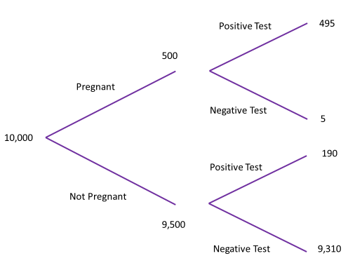
We can now combine all these values to answer the question of the chance a women chosen at random with a negative pregnancy test result is in fact pregnant. The total number of people who had a negative test was 9,315 so gives an overall probability of 93.15% chance that someone chosen at random has a negative pregnancy test result. However, of these only 5 are actually pregnant so the probability a woman chosen at random has a negative pregnancy test but is pregnant is
But what if even though a random person had a negative pregnancy test, they still think they might be pregnant and so mention this to a friend who upon hearing the small probability says that “you had a negative pregnancy test so the probability you’re pregnant is 0.00054, that’s really small” Is the friend correct? The statement the friend made is actually
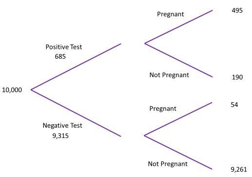
We can now actually calculate the value of
By flipping the tree doing this change in the tree, we’ve used Bayes Theorem to calculate the inverse probability! That is a real wow moment for me. The equation that is used in so many areas of our life can be shown intuitively by flipping a probability tree. If you’re not sure, below is Bayes Theorem for the first probability we calculated and you can see where this and the friend’s statement are shown:
Mixing up the conditional probabilities has become known as the prosecutor’s fallacy, due to its association with miscarriages of justice. Drawing a probability tree is one way of understanding the differences in the two values.

I’m guilty of having made the prosecutor’s fallacy in the past. Not long after my PhD viva I started being sick. There are lots of reasons people are sick: nerves, travel, stomach bug and for me there was also a (very small) chance I was pregnant. After a week or so of being sick I also started feeling dizzy and had a weird taste in my mouth. My pregnancy test was negative. From the above calculations, you can see that if I was the random person selected from the 10,000 people then the probability I was pregnant was very small. However, I wrongly took this to be “I had a negative test therefore the probability I’m pregnant is just as small”
None of the symptoms went away. This is where reasoning under uncertainty and Bayes Theorem come to the fore. I knew it was very unlikely I was pregnant but there was mounting evidence in its favour.
Before the publication of Bayes Theorem, the philosopher David Hume published an essay in which he stated that someone reporting having seen a miracle was not enough evidence to believe that had actually happened. Hume’s reasoning for this was that because miracles are rare and as such are not seen every day, to be convinced that a miracle had happened would need a more evidence.
Religion aside how much evidence do you need to be sure? Countering Hume, Richard Price published and used Bayes Theorem to show that simply having a large amount of counter information (that is lack of miracles not being commonplace) doesn’t remove the chance that the miracle has happened.
Putting these arguments into this context: one side of the argument is that because of the negative pregnancy test the probability I was pregnant was small and as such, a lot more evidence would be needed to be certain I was in fact pregnant. However, countering this was the fact that a negative pregnancy test result didn’t completely remove the probability I was pregnant so this option couldn’t be dismissed.

How much evidence was needed to convince me I was pregnant? The short version is that after a few months I’d had about 10 failed pregnancy tests but was still sick and dizzy. I genuinely sat down with a pen and paper to try and calculate the probability I was pregnant, and this was when I realised that whilst the probability was small I had in fact completed the prosecutor’s fallacy. That was one of many wonderful “oooh” moments maths has given me. Even so I had to fight against the instinct that after so many failed tests in all honesty how could I possibly be pregnant? Well I was (it took a scan to confirm this at which I showed Bayes Theorem to the consultant to explain why I’d kept going back to the doctors) and our house eventually gained the whirlwind of a curly haired daughter we have today.
Probability trees are something lots of people learn at school. They are visual and let you really see the data you’re working with. From them you can calculate conditional probabilities, joint probabilities, flip the tree to calculate inverse probabilities and meet the wonder that is Bayes Theorem and use them to check to see if you’re committing the prosecutor’s fallacy. I think that is pretty impressive.
To me, maths is about solving puzzles and finding patterns. I find solving things I see as being counter intuitive incredibly fun. Whatever maths sparks your interest I genuinely hope you’ve enjoyed the Math Off as much as I have – please go and share your love of maths with others.
So, which pitch did you like the most? Vote now:
Match 27: The final - Sameer Shah vs Sophie Carr
- Sophie with pregnancy tests
- (53%, 810 Votes)
- Sameer with grids
- (47%, 712 Votes)
Total Voters: 1,522
This poll is closed.
Come back tomorrow to find out whether it’s Sameer or Sophie who is the World’s Most Interesting Mathematician!
Update: After a very closely fought match, Sophie is the winner! Congratulations to the World’s Most Interesting Mathematician (2019, of the people I asked to take part and who were free in July), Sophie Carr!
I think that Sophie should work because testing for pregnancy is very important today
I once taught a 20-hour (4 hr/day * 5 days) summer course on the subject of “grids and lattices” (mostly a problem-solving course, but the problems were all based on, and exploited, grid structures in some way.) I wish I’d known about the problem that Sameer presents here.
It was really difficult to choose. I really liked Sameer’s grids and they made me see grids and pixels in an interesting and enjoyable way. But, I just thought that Sophie’s observations had more important implications. Probably totally wrong and I think they both deserve top place. Can’t there be Schrödinger cats solution!
Maths for Sameer Shah
✔️
I am curious if anyone else believes that Sophie’s statement of the problem was incorrect.
First she asks:
What is the probability that a woman chosen at random has a negative pregnancy test and is in fact pregnant?
Then she restates it mathematically:
What we want to calculate is (pregnant|negative test result)
I believe that the correct mathematical way of rendering her original question is:
(pregnant ^ negative test result)
And the answer would then be .0005
If she wanted a question that would be equivalent to:
(pregnant|negative test result)
She should have asked:
If a woman has received a negative result from a pregnancy test, what is the probability that she is pregnant?
Am I correct?
Sophie is my winner as her pitch was on an interesting subject and made sense and has relevance to so many people especially women.
Sophie!
Definitely Sophie.
Sophie Carr’s seems more impactful and relevant in today’s world.
Sameer Shah is my choice
Sameer is enthusiastic about someone else’s brute force solutions… Yes ok the results are entertaining. Sophie is talking about her work on probability which is analytical, deep and very relevant, as her example demonstrates. She wins my vote any day!
Can’t be allowing 1451000 when it should be 145/1000. ;)
Oops! My fault. Fixed now.
Sameer Shah!!
Sophie Carr
Sophie.
Both of these people are geniuses in their own right. I love their passion for mathematics! Shah for the winner for me as he seems to add a note playful nature to a very complex problem.
Sophie Carr. Beautiful pitch & idea!!
Sameer Shah is the Choice.
Voting has closed, but if it hadn’t it would be for Sophie. Contextualising false negative pregnancy test was very interesting!
Sameer shah is my choice
It’s sad that Sophie warns against getting confused by conditional probabilities and herself ends up getting confused. The final frequency trees have to have the same values even if you flip the layers in between. Her calculation of conditional probabilities is also incorrect in many places – P(negative test/pregnant) = 5/500 = 0.01 like she herself assumed in the beginning. I can’t see how the number 54 came into the picture at all – is it a typo? A calculation error on Sophie’s part, I don’t know. I am just sad that something so interesting had to end like this with a mathematically ‘incorrect’ post winning the competition just because it had the better story. Depressing.
I don’t mean to be negative here, but Keshav is exactly right in his comment. Sophie’s story is great, but she over-complicates the math. The “joint frequencies” at the end of the flipped tree should be the same numbers as in the original tree, but moved around. The calculation of 5/9315=0.00054 is actually P(pregnant|negative test)–no further computations need to be performed. Assuming independence of tests, the probability of pregnancy given multiple negative tests is even smaller. A more canonical example of Bayes Theorem and the prosecutor’s fallacy would utilize a much higher misclassification probability when someone is not pregnant.